The demand for computational speed

Overview

Teaching: 0 min
Exercises: 0 min

Questions

Why do we need faster computing platforms?

Objectives

Know standard computational speed measurements

Know representative examples of how large-scale computation servers science, industry, business, and society.

How do we measure speed in computation?

Floating-Point Operation per Second (FLOPS)

Count number of floating-point calculations (arithmetic operations) per second.

Not MIPS (millions of instructions per second) as MIPS also count non-arithmetic operations such as data movement or condition.
$FLOPS = sockets \times \frac{cores}{socket} \times \frac{cycles}{second} \times \frac{FLOPS}{cycle}$

MFLOPS (megaFLOPS) = 1,000,000 FLOPS

GGLOPS (gigaFLOPS) = 1,000,000,000 FLOPS

Modern measurement of speed

TFLOPS (teraFLOPS) = 1,000,000,000,000 FLOPS

Intel’s ASCI Red for Sandia National Laboratory (DOE) was the first supercomputer in the world to achieve 1 TFLOPS in 1997.

ASCI Red is used for large-scale simulation in nuclear weapon development and material analysis.

PFLOPS (petaFLOPS) = 1,000,000,000,000,000 FLOPS

IBM RoadRunner for Los Alamos National Laboratory (DOE) was the first supercomputer to achieve 1 PFLOPS in 2008.

Oak Ridge National Laboratory’s Summit (DOE) is the second fastest supercomputer in the world at 148.6 PFLOPS.

Fugaku of RIKEN Center for Computational Science (Japan) is the current fastest supercomputer at 415 PFLOPS.

EFLOPS (exaFLOPS) = 1,000,000,000,000,000,000 FLOPS

Aurora (> 1 EFLOPS, 2021, Argonne National Lab)

Frontier (> 1.5 EFLOPS, 2021, Oak Ridge National Lab)

El Capitan (> 2 FFLOPS, 2023, Lawrence Livermore National Lab)

Tianhe 3 (first China Exascale computer, 2020, National University of Defense Technology)

Subsequent update to Fugaku (first Japan Exascale computer, 2021, RIKEN Center for Computational Science)

Europe, India, Taiwan on track

The bragging list (The TOP500 Project)

List the 500 most powerful computers in the world.

Count FLOPS by having supercomputer runs well-known computationally intensive tasks

Solve Ax=b, dense random matrix problem.

Primarily dense matrix-matrix multiplications.

Updated twice a year:

International Supercomputing conference (June, Germany)

Supercomputing conference (November, US).

Website: http://www.top500.org

Why do we need this much speed?

The four modern paradigms of science

Theory

Experiment

Simulation

Data analysis

Simulation: study things that are too big, too small, too fast, too slow, too expensive, or too dangerous.

Data anlaysis: study data that are too big, too complex, too fast (streaming data), too noisy.

Faster computer gives more details

Hurricane Sandy (2012)

the deadliest and most destructive, as well as the strongest hurricane of the 2012 Atlantic hurricane season,

the second-costliest hurricane on record in the United States (nearly $70 billion in damage in 2012),

affected 24 states, with particularly severe damage in New Jersey and New York,

hit New York City on October 29, flooding streets, tunnels and subway lines and cutting power in and around the city.

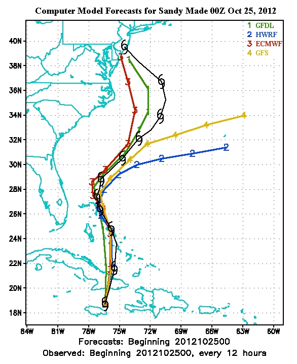
Various forecasts of Sandy

Geophysical Fluid Dynamic Laboratory hurricane model (National Oceanic and Atmostpheric Administration)

Hurricane Weather Resaarch and Forecasting model (NOAA/Naval Research Laboratory/Florida State University)

European Centre for Medium Range Weather Forecast model (ECMWF)

Global Forecast Model (National Weather Service)

Which model is closest to reality?

One of the contributing factors

http://blogs.agu.org/wildwildscience/2013/02/17/seriously-behind-the-numerical-weather-prediction-gap/

The US has catched up

NOAA Weather Computer upgrade

Two new supercomputers, Luna and Surge

2.89 PFLOPS each for a total of 5.78 PFLOPS (previous generation is only 776 TFLOPS)

Increase water quantity forecast from 4000 locations to 2.7 million locations (700-fold increase in spatial density)

Can track and forecast 8 storms at any given time

44.5 million dollars investment

Covid and HPC

US HPC Consortium to contribute to Covid research

Toward explaining signs of COVID symptoms

Many other work (published in Nature) include supercomputing usages for molecular dynamic simulation/data analysis.

Manufacturing and HPC

For 767 development, Boeing built and tested 77 physical prototypes for wing design.

For 787 development, only 11 prototypes were built.

Optimized via more than 800,000 hours of computer simulation.

Oil and Gas Expoloration improvement with HPC

Los Alamos National Lab

Development of large-scale data analytic techniques to simulate and predict subsurface fluid distribution, temperature, and pressure

This reduces the need for observation wells (has demonstrated commercial success)

Fraud Detection at PayPal

10M+ logins, 13M+ transactions, 300 variables per events

~4B inserts, ~8B selects

MPI-like applications, Lustre Parallel File Systems, Hadoop Saved over $700M in fraudulent transactions during first year of deployment

Key Points

Computational speed is critical in solving humanity’s growing complex problems across all aspects of society.

Introduction to paralel and distributed computing

Overview

Teaching: 0 min
Exercises: 0 min

Questions

What is parallel computing?

Objectives

Understand basic architectures and computing models for parallel computing.

Understand and be able to carry out rudimentary speedup and efficiency study.

Envision the payroll problem

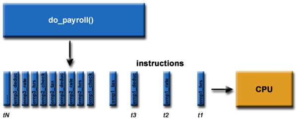
Components of a computation problem

Computational task

Execution framework.

Computing resources.

Parallelizing payroll

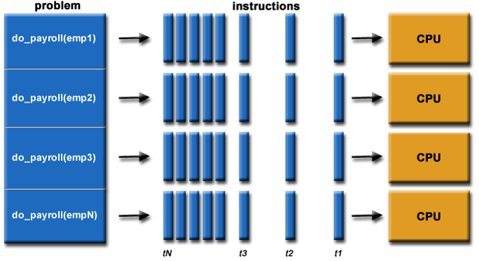
Computational tasks should be able to …

Be borken apart into discrete pieces of work that can be solved simultaneously.

Be solved in less time with multiple computing resources than with a single computing resource.

Execution framework should be able to …

Execute multiple program instructions concurrently at any moment in time

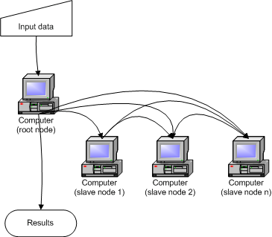
Computing resources might be …

A single computer with multiple processors.

An arbitrary number of computers connected by a network.

A special computational component inside a single computer, separate from the main processors (GPU), or

Any combintations of the above.

The progress

How do parallel and distributed computing resources evolve?

Single site, single computer, single core

Single site, single computer, multiple cores

Single site, multiple computers, multiple cores

Multiple sites, multiple computers, multiple cores, federated domains

Multiple site, multiple computers, multiple cores, virtula unified domain

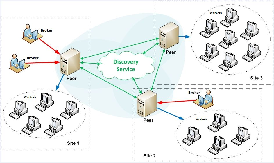
Distributed computing systems

“A collection of individual computing devices that can communicate with each other.” (Attiya and Welch, 2004).

emphasis …

“A collection of individual computing devices that can communicate with each other.” (Attiya and Welch, 2004).

Can we just throw more computers at the problem?

Parallel speedup: how much faster the program becomes once some computing resources are added.

Parallel efficiency: Ratio of performance improvement per individual unit of computing resource.

Parallel speedup

Given p processors,

Speedup, S(p), is the ratio of the time it takes to run the program using a single processor over the time it takes to run the program using p processors.

The time it takes to run the program using a single processor, $t_{s}$ : sequential run time

The time it takes to the the program using multiple processor, $t_{p}$ : parallel run time $\\\\S(p) = \frac{sequential\ run\ time}{parallel\ run\ time} = \frac{t_s}{t_p}\\$

Example 1

A program takes 30 seconds to run on a single-core machine and 20 seconds to run on a dual-core machine. What is the speedup of this program?

Solution

$t_s=30$
$t_p=20$
$S=\frac{t_s}{t_p}=\frac{30}{20}=1.5$

Theoretical max

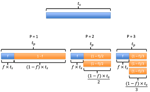
Let f be the fraction of the program that is not parallelizable.

Assume no overhead.

Running the program using one processor will take time $t_s$ .

The parallel run time, $t_p$ , can be calculated as the time it take to run the fraction that is non-parallelizable ( $f\times t_s$ ) plus the remainning parallelizable fraction ( $1-f$ ).

If $p=1$ , this simplifies to $t_p=f\times t_s + (1-f)\times t_s$ .

Assume no overhead, this means that we reduce the speed by half as we double the number of processor.

And so on …

Amdahl’s Law

This brings us to Amdahl’s Law, which quantifies speedup in term of number of processors and fraction of non-parallelizable code:
$S(p)=\frac{t_s}{t_p}=\frac{t_s}{f\times t_s + (1-f)\times t_s}=\frac{1}{f + \frac{1-f}{p}}=\frac{p}{f \times (p-1) + 1}$

Parallel efficiency

The efficiency E is then defined as the ratio of speedup S(p) over the number of processors p.
$E=\frac{\frac{p}{f \times (p-1) + 1}}{p}=\frac{1}{f \times (p-1) + 1}$

E is often measured as percentage.

For example, E = 0.8 means the parallel efficiency is 80%.

Example 2

Suppose that 4% of my application is serial. What is my predicted speedup according to Amdahl’s Law on 5 processors?

Solution

$f=0.04$
$p=5$
$S=\frac{p}{(p-1)f + 1}=\frac{5}{4 \times 0.4 +1}=1.9231$

Example 3

Suppose that I get a speedup of 8 when I run my application on 10 processors. According to Amdahl’s Law:

What portion of my code is serial?

What is the speedup on 20 processors?

What is the efficiency on 5 processors? 20 processors?

What is the best speedup that I could achieve?

Serial portion

$S=8$
$p=10$
$S=\frac{p}{(p-1)f + 1}$
$8=\frac{10}{9f+1}$
$9f + 1 = \frac{10}{8}$
$f=\frac{1}{36}$

Speedup on 20 processors

$f=\frac{1}{36}$
$p=20$
$S_{20}=\frac{p}{(p-1)f + 1}=\frac{20}{\frac{19}{36}+1} \approx 13.0909$

Efficiency

$E=\frac{1}{(p-1)f + 1}$
$E_5=\frac{1}{\frac{4}{36}+1} = 90\%$
$E_{20}=\frac{1}{\frac{19}{36} + 1} \approx 65.45\%$

Best speedup

$f=\frac{1}{36}$
$S_{\infty}=\lim_{p \to +\infty} \frac{p}{(p-1)f + 1} = \lim_{p \to +\infty} \frac{1}{\frac{p}{p-1}f + \frac{1}{p}}=\frac{1}{f}$
$S_{\infty}= 36$

In other word, the highest number of processors one should add to this problem is 36.

Limiting factors of parallel speedup

Non-parallelizable code.

Communication overhead.

If there is no limiting factor …

0% non-paralellizable code.

No communication overhead.
$S_{\infty}=\lim_{f \to 0} \frac{p}{(p-1)f + 1} = p$
$S \leq p$

Superlinear speedup

The unicorn of parallel and distributed computing.

Poor sequential reference implementation.

Memory caching.

I/O blocking.

Computer architecture: Flynn’s Taxonomy

Types of distributed computing systems

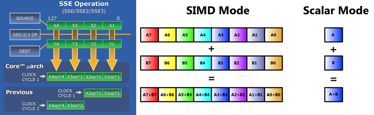
Streaming SIMD extensions for x86 architectures.

Shared memory.

Distributed shared memory.

Heterogeneous computing (accelerators).

Message passing.

Streaming SIMD

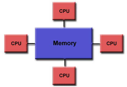
Shared memory

One processor, multiple threads.

All threads have read/write access to the same memory.

Programming models:

Threads (pthread) - programmer manages all parallelism.

OpenMP: compiler extensions handle.

Vendor libraries: (Intel MKL - math kernel libraries)

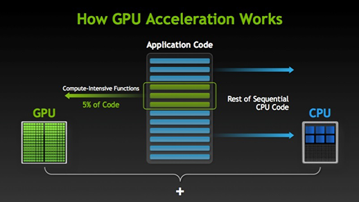
Heterogeneous computing

GPU

FPGA

Co-processors

GPU - graphics processing unit

Processor unit on graphic cards designed to support graphic rendering (numerical manipulation).

Significant advantage for certain classes of scientific problems.

Programming models:

CUDA: Library developed by NVIDIA for their GPUs.

OpenACC: Standard developed by NVIDIA, Cray, and Portal Compiler (PGI).

OpenAMP: Extension to Visual C++ to direct computation to GPU.

OpenCL: Public standard by the group the developed OpenGL.

FPGA - field programmable array

Dynamically reconfigurable circuit board.

Expensive, difficult to program.

Power efficient, low heat.

Co-processors

Enables offloading of computationally intensive tasks from main CPU.

Similar to GPU, but can support a wider range of computational tasks.

Intel

Xeon Phi processor line.

PCIe-based add-on cards, but could also be used as a stand alone CPU.

Unlike GPU, Intel Xeon supports all programs targeted to standard x86 CPU (very minor modification if any)

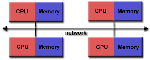
Message passing distributed computing

Processes handle their own memory.

Data is passed between processes via messages.

Scales well.

Cluster can be built from commodity parts.

Cluster can easily be expanded.

Cluster can be heterogeneous.

Programming models:

MPI: standardized message passing library.

MPI + OpenMP: hybrid model.

MapReduce programming model for big data processing.

Benchmarking

LINPACK (Linear Algebra Package): Dense Matrix Solver

HPCC: High-Performance Computing Challenge.

HPL (LINPACK to solve linear system of equations)

DGEMM (Double precision general matrix multiply)

STREAM (Memory bandwidth)

PTRANS (Parallel matrix transpose to measure processors communication)

RandomAccess (random memory updates)

FFT (double precision complex discrete fourier transform)

Communication bandwidth and latency

SHOC: Scalable heterogeneous computing

Non-traditional system (GPU)

TestDFSIO

I/O performance of MapReduce/Hadoop Distributed File System.

Ranking

TOP500: Rank the supercomputers based on their LINPACK score.

GREEN500: Rank the supercomputers with emphasis on energy usage (LINPACK/power consumption).

GRAPH500: Rank systems based on benchmarks designed for data-intensive computing.

Key Points

There various parallel computing architecture/model

Users need to find the one that give the best speedup/efficiency measures.

Speed/efficiency depends on how well programs are parallelized.

Introduction to OpenMP

Overview

Teaching: 0 min
Exercises: 0 min

Questions

What is the OpenMP model?

Objectives

Know the target hardware architecture for OpenMP

Be able to compile and run an OpenMP program.

Understand the concept of parallel regions.

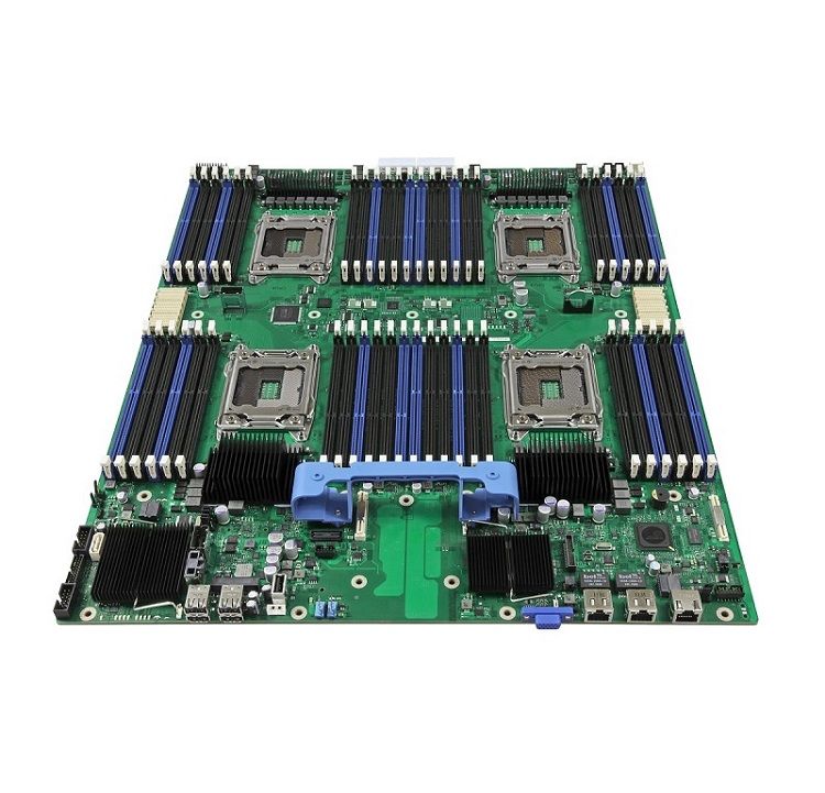
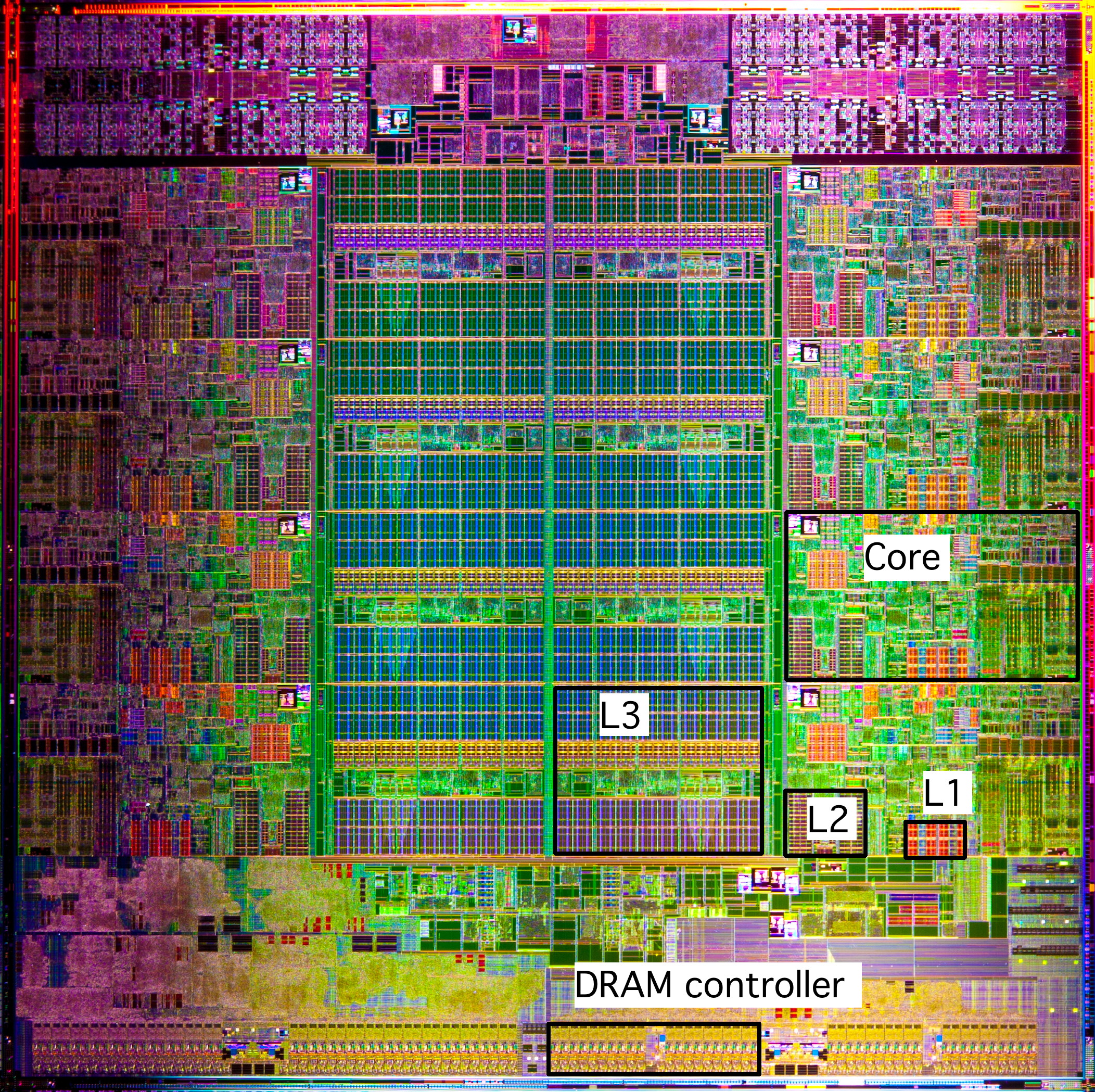
Target hardware

Single computing node, multiple sockets, multiple cores.

Dell PowerEdge M600 Blade Server.

Intel Sandy Bridge CPU.

In summary

Node with up to four sockets.

Each socker has up to 60 cores.

Each core is an independent CPU.

Each core has access to all the memory on the node.

Target software

Provide wrappers for threads and fork/join model of parallelism.

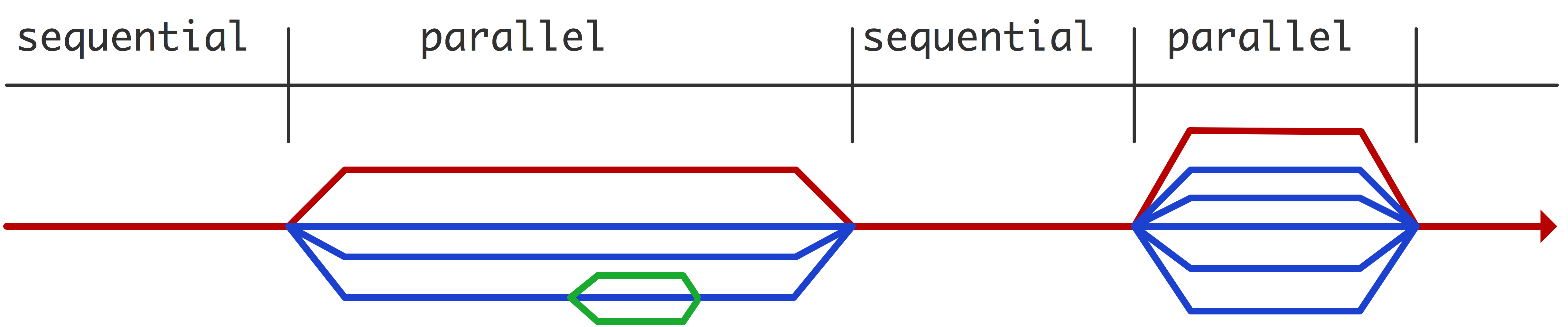
Program originally runs in sequential mode.

When parallelism is activated, multiple threads are forked from the original proces/thread (master thread).

Once the parallel tasks are done, threads are joined back to the original process and return to sequential execution.

The threads have access to all data in the master thread. This is shared data.

The threads also have their own private memory stack.

Basic requirements to write, compile, and run an OpenMP program

Source code (C) needs to include #include <omp.h>

Compiling task need to have -fopenmp flag.

Specify the environment variable OMP_NUM_THREADS.

OMP directives
OpenMP must be told when to parallelize.
For C/C++, pragma is used to annotate:
#pragma omp somedirective clause(value, othervalue)
parallel statement;
or
#pragma omp somedirective clause(value, othervalue)
{
parallel statement 1;
parallel statement 2;
...
}

Hands-on 1: Setup directory
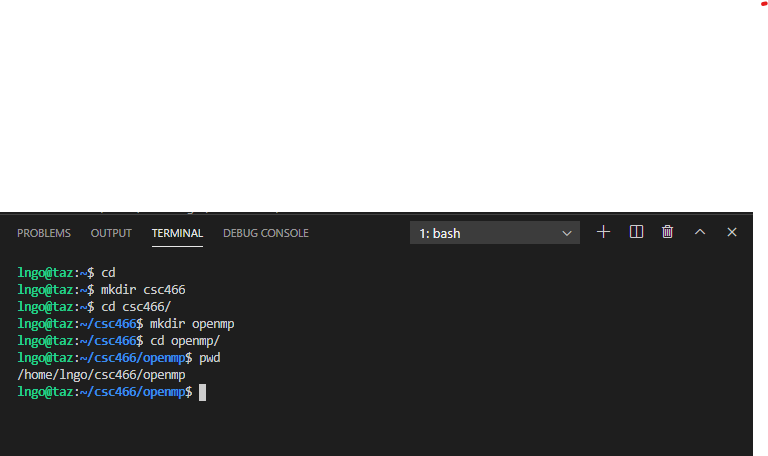
Create a directory named csc466 inside your home directory, then change into that directory.
Next, create a directory called openmp, and change into that directory
$ cd
$ mkdir csc466
$ cd csc466
$ mkdir openmp
$ cd openmp

Hands-on 2: Create hello_omp.c

In the EXPLORER window, right-click on csc466/openmp and select New File.

Type hello_omp.c as the file name and hits Enter.

Enter the following source code in the editor windows:

Save the file when you are done:

Ctrl-S for Windows/Linux

Command-S for Macs

Memorize your key-combos!.
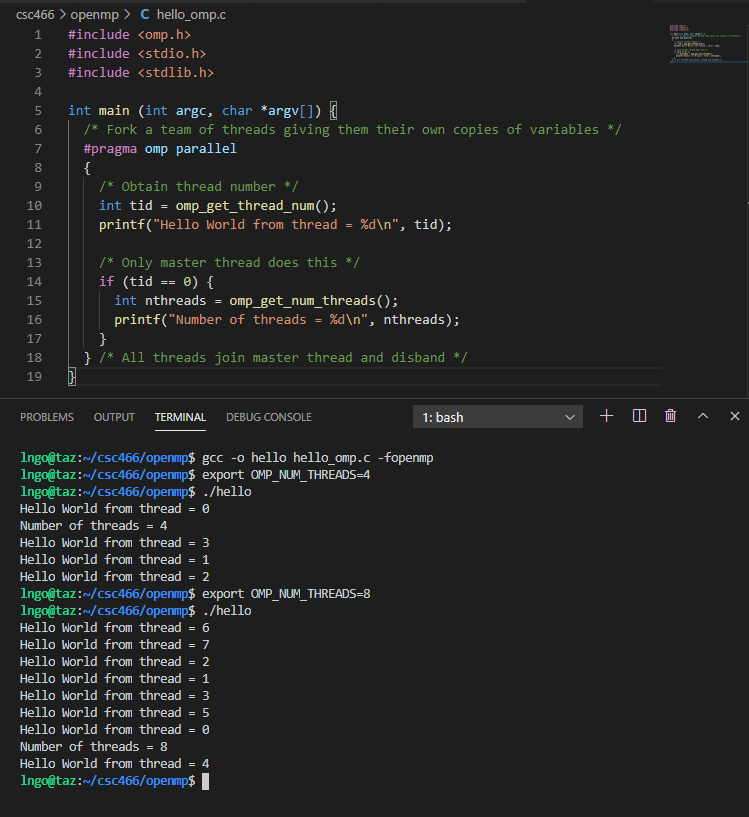
#include <omp.h>
#include <stdio.h>
#include <stdlib.h>

int main (int argc, char *argv[]) {
  /* Fork a team of threads giving them their own copies of variables */
  #pragma omp parallel 
  {
    /* Obtain thread number */
    int tid = omp_get_thread_num();
    printf("Hello World from thread = %d\n", tid);

    /* Only master thread does this */
    if (tid == 0) {
      int nthreads = omp_get_num_threads();
      printf("Number of threads = %d\n", nthreads);
    }
  } /* All threads join master thread and disband */
}
Line 1: Include omp.h to have libraries that support OpenMP.

Line 7: Declare the beginning of the parallel region. Pay attention to how the curly bracket is setup, comparing to the other curly brackets.

Line 10: omp_get_thread_num gets the ID assigned to the thread and then assign it to a variable named tid of type int.

Line 15: omp_get_num_threads gets the value assigned to OMP_NUM_THREADS and return it to a variable named nthreads of type int.

What’s important?

tid and nthreads.

They allow us to coordinate the parallel workloads.

Specify the environment variable OMP_NUM_THREADS.
$ export OMP_NUM_THREADS=4

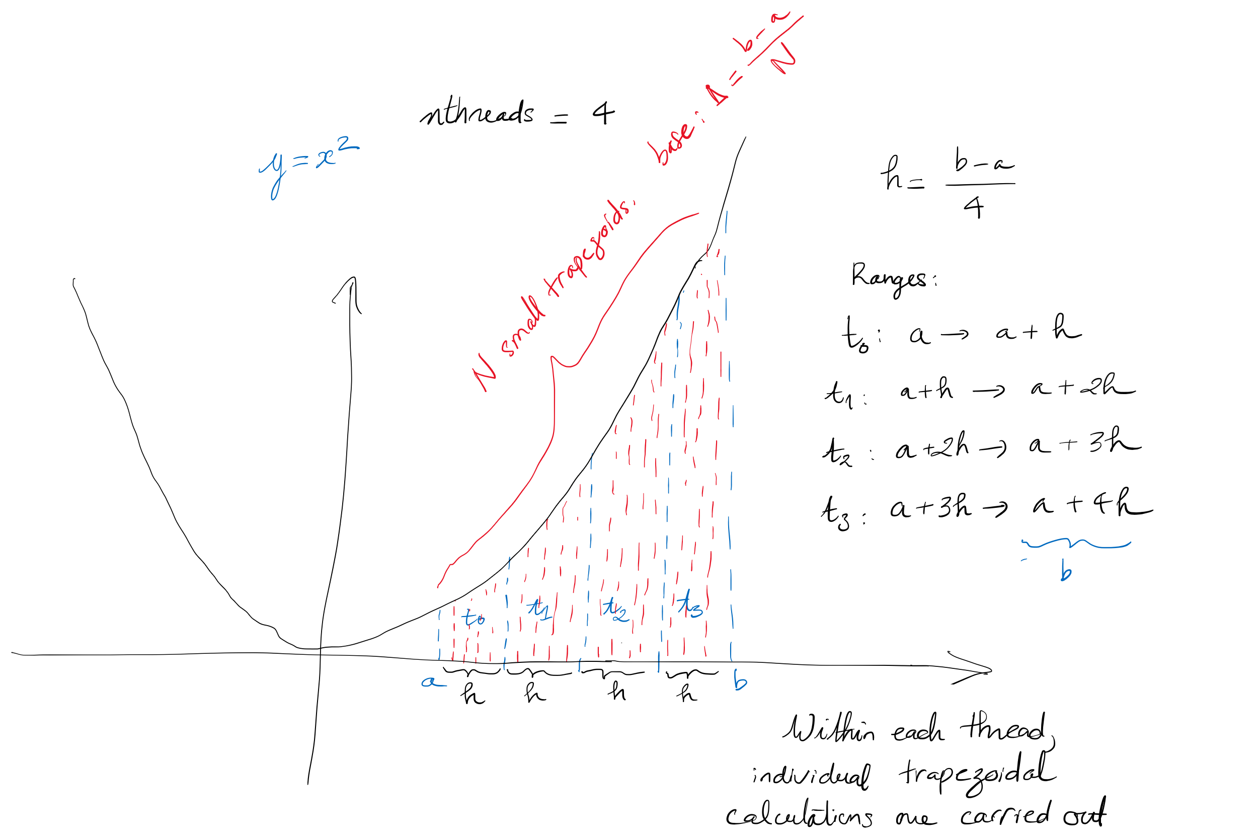
Example: trapezoidal

Problem: estimate the integral of $y=x^2$ on $[2,8]$ using trapezoidal rule. four threads.

With 4 threads: nthreads=4.

How to decide which thread will handle which segment?

How to get all results back together?

Hands-on 3: Trapezoid implementation

In the EXPLORER window, right-click on csc466/openmp and select New File.
Type trapezoid.c as the file name and hits Enter.
Enter the following source code in the editor windows:
Save the file when you are done:
- Ctrl-S for Windows/Linux
- Command-S for Macs
Memorize your key-combos!.

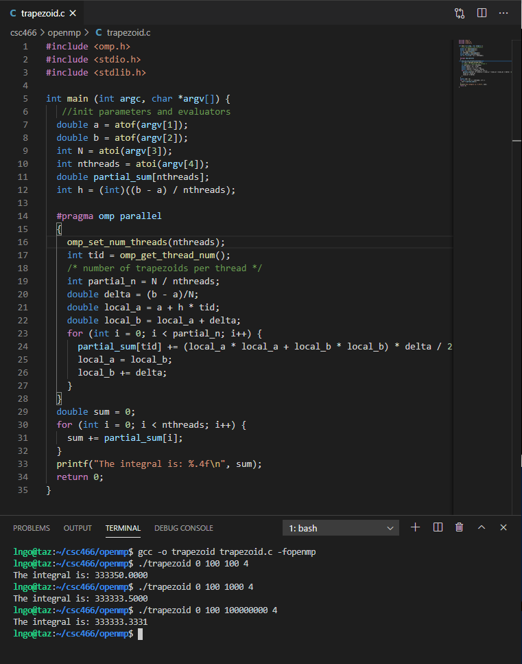
#include <omp.h>
#include <stdio.h>
#include <stdlib.h>

int main (int argc, char *argv[]) {
  //init parameters and evaluators
  double a = atof(argv[1]);
  double b = atof(argv[2]);
  int N = atoi(argv[3]);
  int nthreads = atoi(argv[4]);
  double partial_sum[nthreads];
  double h = ((b - a) / nthreads);    

  omp_set_num_threads(nthreads);
  #pragma omp parallel 
  {
    int tid = omp_get_thread_num();
    /* number of trapezoids per thread */
    int partial_n = N / nthreads;
    double delta = (b - a)/N;
    double local_a = a + h * tid;
    double local_b = local_a + delta;
    for (int i = 0; i < partial_n; i++) {
      partial_sum[tid] += (local_a * local_a + local_b * local_b) * delta / 2;
      local_a = local_b;
      local_b += delta;
    }
  } 
  double sum = 0;
  for (int i = 0; i < nthreads; i++) {
    sum += partial_sum[i];
  }
  printf("The integral is: %.4f\n", sum);
  return 0;
}

create trapezoid.c

Hands-on 4: A bit more detailed

Modify the trapezoid.c so that it looks like below.
Save the file when you are done:
- Ctrl-S for Windows/Linux
- Command-S for Macs
Memorize your key-combos!.

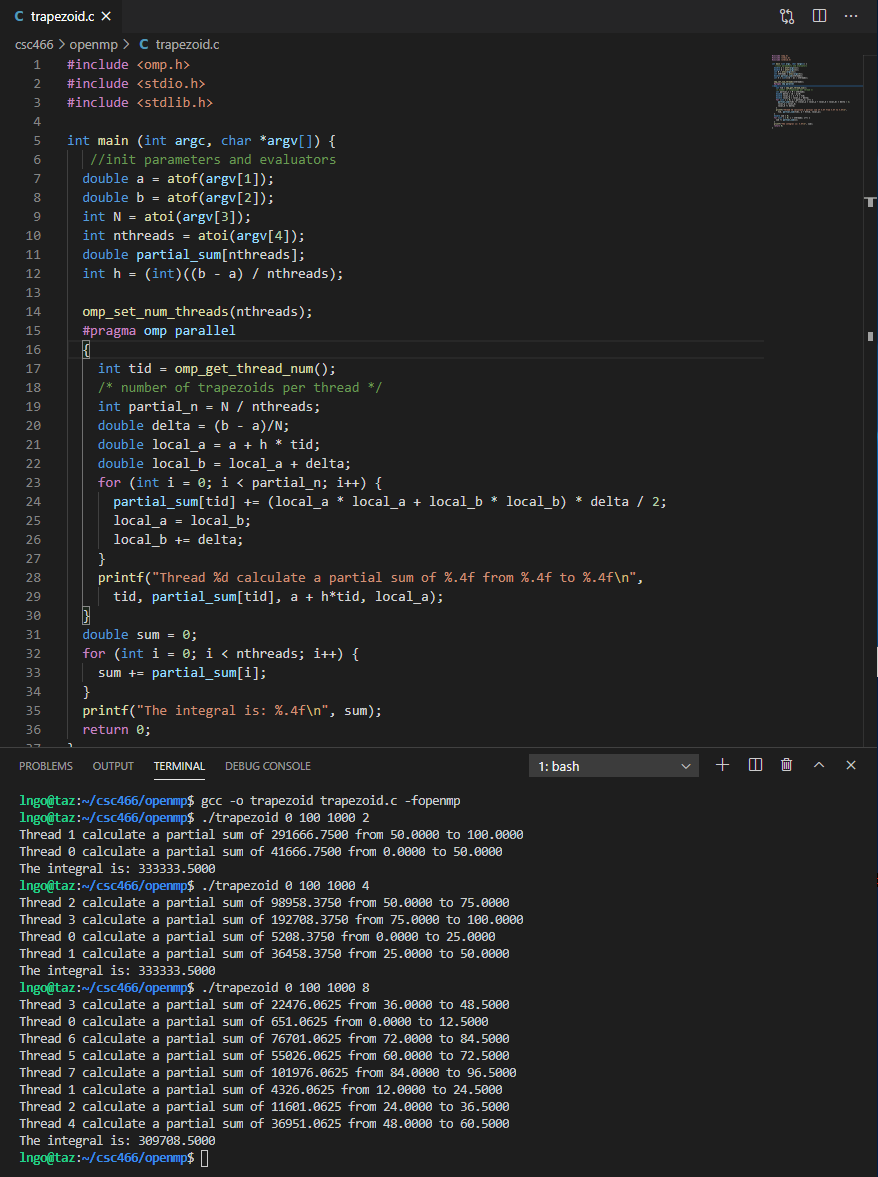
#include <omp.h>
#include <stdio.h>
#include <stdlib.h>

int main (int argc, char *argv[]) {
  //init parameters and evaluators
  double a = atof(argv[1]);
  double b = atof(argv[2]);
  int N = atoi(argv[3]);
  int nthreads = atoi(argv[4]);
  double partial_sum[nthreads];
  double h = ((b - a) / nthreads);    

  omp_set_num_threads(nthreads);
  #pragma omp parallel 
  {
    int tid = omp_get_thread_num();
    /* number of trapezoids per thread */
    int partial_n = N / nthreads;
    double delta = (b - a)/N;
    double local_a = a + h * tid;
    double local_b = local_a + delta;
    for (int i = 0; i < partial_n; i++) {
      partial_sum[tid] += (local_a * local_a + local_b * local_b) * delta / 2;
      local_a = local_b;
      local_b += delta;
    }
    printf("Thread %d calculate a partial sum of %.4f from %.4f to %.4f\n", tid, partial_sum[tid], a + h*tid, local_a);
  } 
  double sum = 0;
  for (int i = 0; i < nthreads; i++) {
    sum += partial_sum[i];
  }
  printf("The integral is: %.4f\n", sum);
  return 0;
}

modify trapezoid.c

Challenge 1:

Alternate the trapezoid.c code so that the parallel region will invokes a function to calculate the partial sum.

Solution

#include <omp.h>
#include <stdio.h>
#include <stdlib.h>

double trap(double a, double b, int N, int nthreads, int tid) {
  double h = ((b - a) / nthreads);  
  int partial_n = N / nthreads;
  double delta = (b - a)/N;
  double local_a = a + h * tid;
  double local_b = local_a + delta;
  double p_sum = 0;
  for (int i = 0; i < partial_n; i++) {
    p_sum += (local_a * local_a + local_b * local_b) * delta / 2;
    local_a = local_b;
    local_b += delta;
  }
  return p_sum;
}

int main (int argc, char *argv[]) {
   //init parameters and evaluators
  double a = atof(argv[1]);
  double b = atof(argv[2]);
  int N = atoi(argv[3]);
  int nthreads = atoi(argv[4]);
  double partial_sum[nthreads];

  omp_set_num_threads(nthreads);
  #pragma omp parallel 
  {
    int tid = omp_get_thread_num();
    partial_sum[tid] = trap(a, b, N, nthreads, tid) ;
  } 
  double sum = 0;
  for (int i = 0; i < nthreads; i++) {
    sum += partial_sum[i];
  }
  printf("The integral is: %.4f\n", sum);
  return 0;
} 

Challenge 2:

Write a program called sum_series.c that takes a single integer N as a command line argument and calculate the sum of the first N non-negative integers.
Speed up the summation portion by using OpenMP.
Assume N is divisible by the number of threads.

Solution

#include <omp.h>
#include <stdio.h>
#include <stdlib.h>

int sum(int N, int nthreads, int tid) {
  int count = N / nthreads;  
  int start = count * tid + 1;
  int p_sum = 0;
  for (int i = start; i < start + count; i++) {
    p_sum += i;
  }
  return p_sum;
}

int main (int argc, char *argv[]) {
  int N = atoi(argv[1]);
  int nthreads = atoi(argv[2]);
  int partial_sum[nthreads];
   
  omp_set_num_threads(nthreads);
  #pragma omp parallel 
  {
    int tid = omp_get_thread_num();
    partial_sum[tid] = sum(N, nthreads, tid) ;
  } 
  int sum = 0;
  for (int i = 0; i < nthreads; i++) {
    sum += partial_sum[i];
  }
  printf("The sum of series is: %.4f\n", sum);
  return 0;
} 

Challenge 3:

Write a program called sum_series_2.c that takes a single integer N as a command line argument and calculate the sum of the first N non-negative integers.
Speed up the summation portion by using OpenMP.
There is no assumtion that N is divisible by the number of threads.

Solution

#include <omp.h>
#include <stdio.h>
#include <stdlib.h>

int sum(int N, int nthreads, int tid) {
  int count = N / nthreads;  
  int start = count * tid;
  int end = start + count;
  int p_sum = 0;

  for (int i = start; i < end; i++) {
    p_sum += i;
  } 
  if (tid < remainder) {
    p_sum += count * remainder + tid + 1;
  }

  return p_sum;
}

int main (int argc, char *argv[]) {
  int N = atoi(argv[1]);
  int nthreads = atoi(argv[2]);
  int partial_sum[nthreads];
   
  omp_set_num_threads(nthreads);
  #pragma omp parallel 
  {
    int tid = omp_get_thread_num();
    partial_sum[tid] = sum(N, nthreads, tid) ;
  } 
  int sum = 0;
  for (int i = 0; i < nthreads; i++) {
    sum += partial_sum[i];
  }
  printf("The sum of series is: %.4f\n", sum);
  return 0;
} 

Hands-on 5: Trapezoid implementation with timing

In the EXPLORER window, right-click on csc466/openmp and select New File.
Type trapezoid_time.c as the file name and hits Enter.
Enter the following source code in the editor windows (You can copy the contents of trapezoid.c with function from Challenge 1 as a starting point):
Save the file when you are done:
- Ctrl-S for Windows/Linux
- Command-S for Macs
Memorize your key-combos!.

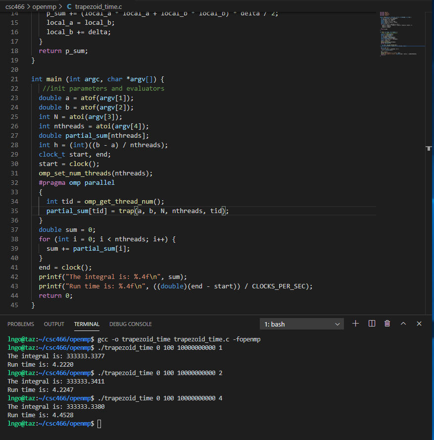
#include <omp.h>
#include <stdio.h>
#include <stdlib.h>
#include <time.h>

int main (int argc, char *argv[]) {
  //init parameters and evaluators
  double a = atof(argv[1]);
  double b = atof(argv[2]);
  int N = atoi(argv[3]);
  int nthreads = atoi(argv[4]);
  double partial_sum[nthreads];
  double h = ((b - a) / nthreads);  
  clock_t start, end;  

  omp_set_num_threads(nthreads);
  start = clock();
  #pragma omp parallel 
  {
    int tid = omp_get_thread_num();
    /* number of trapezoids per thread */
    int partial_n = N / nthreads;
    double delta = (b - a)/N;
    double local_a = a + h * tid;
    double local_b = local_a + delta;
    for (int i = 0; i < partial_n; i++) {
      partial_sum[tid] += (local_a * local_a + local_b * local_b) * delta / 2;
      local_a = local_b;
      local_b += delta;
    }
  } 
  end = clock();
  double sum = 0;
  for (int i = 0; i < nthreads; i++) {
    sum += partial_sum[i];
  }
  printf("The integral is: %.4f\n", sum);
  printf("The run time is: %.4f\n", ((double) (end - start)) / CLOCKS_PER_SEC);
  return 0;
}

create trapezoid.c

How’s the run time?

Key Points

Introduction to XSEDE

Overview

Teaching: 0 min
Exercises: 0 min

Questions

What is XSEDE?

Objectives

Know the history, organization, and impact of XSEDE

Be able to access one XSEDE resource

XSEDE

Extreme Science and Engineering Discovery Enrironment

2011 - now

17 institutions at the beginning.

Successor of the TeraGrid program

2001 - 2011.

9 sites (UIUC, SDSC, ANL, CalTech, PSC, ORNL, Purdue, Indiana, TACC)

Unit of computation: SU (Service Unit)

1 SU = 1 core-hour of computing time.

What is currently part of XSEDE

Stampede2 (TACC): 18 PFLOPS

4,200 Intel Knights Landing (68 cores), 96GB memory

1,736 Intel Xeon Skylake (48 cores), 192GB memory.

31 PB storage.

Comet (SDSC): 2.76 PFLOPS

1944 Intel Haswell (24 cores), 320 GB memory.

72 Intel Haswell (24 cores) with GPUs (36 K80, 36 P100), 128GB memory.

4 large memory nodes (1.5TB memory each), Intel CPU (64 cores).

7.6 PB storage.

Bridges (PSC) - we use this.

752 Intel Haswell (28 cores), 128GB memory.

42 Intel Broadwell (36-40 cores), 3TB memory.

4 Intel Broadwell (36-40 cores), 12 TB memory.

16 Haswell nodes with dual K80 GPU, 32 Haswell nodes with dual P100 GPU.

9 Intel Skylake nodes with 8 V100 GPUs per node, 128GB memory.

1 DGX-2 (Intel Cascadelake) with 16 V100 GPU, 1.5 TB memory.

Jetstream (IU)

Cloud provider (baremetal) for academic research and education.

640 nodes, totaling 7680 cores, 40TB memory, and 640 TB local storage.

What will be part of XSEDE in the next five years?

Jetstream2 (IU) - $10M

Predicted to be 8 PFLOPS.

$10M.

Delta (NCSA) - $10M

TBD

Anvil (Purdue) - $10M

1,000 AMD Epyc Milan (128 cores), 256GB memory.

32 AMD Epyc Milan (128 cores), 1TB memory

16 AMD Epyc Milan (128 cores), 256GB memory, 4 NVIDIA A100 GPUs.

Neocortex (PSC) - $5M.

Special purpose supercomputer built to support AI research.

2 Cerebras CS-1: largest chip ever built with 400,000 cores, 16GB on-chip memory, and 9.6PB/s memory bandwidth.

1 HPE Superdome gateway: 24 TB memory, 204.6 local storage, 24 100GB network cards, 16 Infiniband network cards.

Voyager (SDSC) - $5M.

TBD.

What do we have access to?

50,000 SUs on Bridges RSM.

500GB total storage on Bridges Pylon.

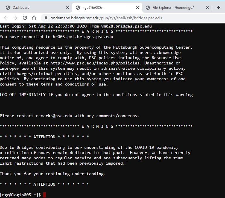
Hands-on 1: Login to PSC Bridges

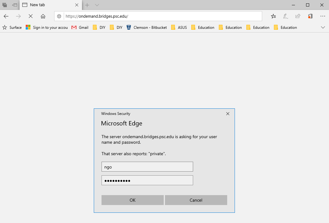
Open a browser and go to https://ondemand.bridges.psc.edu.

Enter the Bridges user name and password from the confirmation email.

Hands-on 2: Login to PSC Bridges

Open a browser and go to https://ondemand.bridges.psc.edu.

Enter the Bridges user name and password from the confirmation email.

Hands-on 3: OnDemand navigation

Click on the Files and then Home Directory.

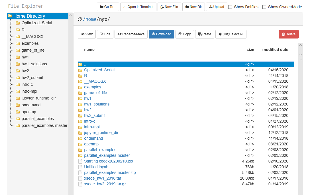
Top button row (Go To, Open in Terminal, New File, New Dir, Upload) operates at directory level.

Next row (View, Edit, Rename/Move, Copy, Paste) operates on files.

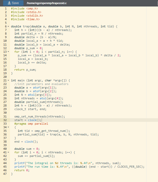
Hands-on 4: Trapezoid implementation with timing

Click New Dir and enter openmp. Hit OK.

Create the openmp directory

Double click on openmp.
Click New File and enter trapezoid.c. Hit OK.
Select trapezoid.c and click Edit.
Type/copy the code from the below into the editor windows.
Click Save to save the file.

#include <omp.h>
#include <stdio.h>
#include <stdlib.h>
#include <time.h>

double trap(double a, double b, int N, int nthreads, int tid) {
  double h = ((b - a) / nthreads);  
  int partial_n = N / nthreads;
  double delta = (b - a)/N;
  double local_a = a + h * tid;
  double local_b = local_a + delta;
  double p_sum = 0;
  for (int i = 0; i < partial_n; i++) {
    p_sum += (local_a * local_a + local_b * local_b) * delta / 2;
    local_a = local_b;
    local_b += delta;
  }
  return p_sum;
}

int main (int argc, char *argv[]) {
  //init parameters and evaluators
  double a = atof(argv[1]);
  double b = atof(argv[2]);
  int N = atoi(argv[3]);
  int nthreads = atoi(argv[4]);
  double partial_sum[nthreads];
  clock_t start, end;  

  omp_set_num_threads(nthreads);
  start = clock();
  #pragma omp parallel 
  {
    int tid = omp_get_thread_num();
    partial_sum[tid] = trap(a, b, N, nthreads, tid);
    printf("Thread %d has partial sum %f\n", tid, partial_sum[tid]);
  } 
  end = clock();
  double sum = 0;
  for (int i = 0; i < nthreads; i++) {
    sum += partial_sum[i];
  }
  printf("The integral is: %.4f\n", sum);
  printf("The run time is: %.4f\n", ((double) (end - start)) / CLOCKS_PER_SEC);
  return 0;
}

Editingg trapezoid.c

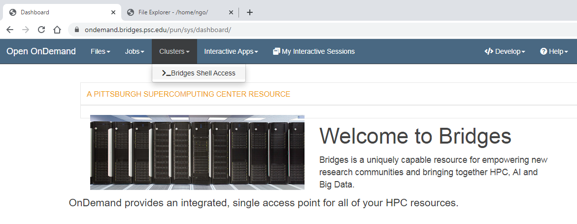
Hands-on 5: Bridges shell access

Go back to the Open OnDemand tab and navigate to Bridges Shell Access under Clusters

This enables an in-browser terminal to a virtual login VM on bridges

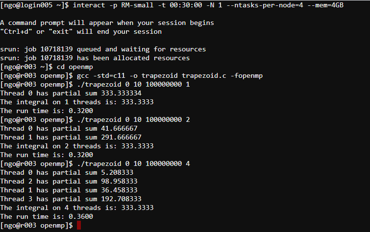
Hands-on 6: Requesting interactive allocation on Bridges

Login node = lobby.

We need to request resources to run jobs.

interact: request an interactive allocation

-p: partition requested (always RM or RM-small)

-t: duration (HH:MM:SS)

-N: number of nodes (chunks)

--ntasks-per-node: number of threads/cores per node (per chunk)

--mem: amount of memory requested.
$ interact -p RM-small -t 00:30:00 -N 1 --ntasks-per-node=4 --mem=4GB
$ cd openmp
$ gcc -std=c11 -o trapezoid trapezoid.c -openmp
$ ./trapezoid 0 10 100000000 1
$ ./trapezoid 0 10 100000000 2
$ ./trapezoid 0 10 100000000 4
What is the problem?

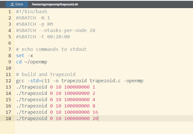
Hands-on 7: Submitting batch job on Bridges

For long running jobs.

Switch to File Exporer tab.

Inside openmp, Click New File and enter trapezoid.sh. Hit OK.

Type/copy the code from the below into the editor windows.

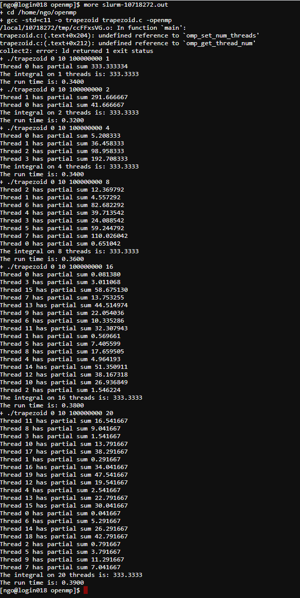
Click Save to save the file.
#!/bin/bash
#SBATCH -N 1
#SBATCH -p RM
#SBATCH --ntasks-per-node 28
#SBATCH -t 00:20:00

# echo commands to stdout 
set -x
cd ~/openmp

# build and trapezoid
gcc -std=c11 -o trapezoid trapezoid.c -openmp
./trapezoid 0 10 100000000 1
./trapezoid 0 10 100000000 2
./trapezoid 0 10 100000000 4
./trapezoid 0 10 100000000 8
./trapezoid 0 10 100000000 16
./trapezoid 0 10 100000000 20
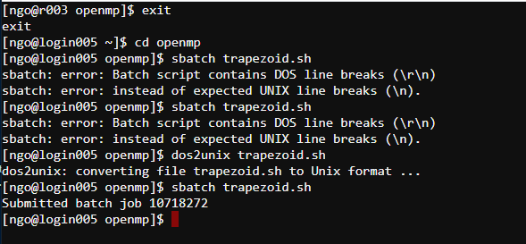
To submit the batch script:

This must be done on the login node. If you are still on an r node, need to exit back to a login node.
$ cd openmp
$ sbatch trapezoid.sh
Be careful with copy/pasting.

Use dos2unix to remove DOS line breaks if that happens.

Check job status using squeue -u $USER

See SLURM’s squeue document page for status codes.

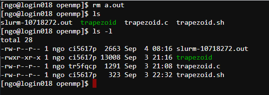
An output report file will be created. The filename format is slurm-JOBID.out

Uses more to view the content of the output file. You can also use Edit or View to view this file on the File Explorer tab.

The professor made a mistake in the submission script. What is it?

Why does the program still run even though there was an error in the gcc command?

Key Points

OpenMP: parallel regions and loop parallelism

Overview

Teaching: 0 min
Exercises: 0 min

Questions

Do we have to manually do everything?

Objectives

Know how to use parallel for pragma

Loop parallelism

Very common type of parallelism in scientific code

In previous trapezoid example, we calculate the division of iteration manually.

An alternative is to use parallel for pragma

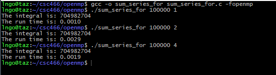
Hands-on 1: Sum series implementation

In the EXPLORER window, right-click on csc466/openmp and select New File.
Type sum_series_for.c as the file name and hits Enter.
Enter the following source code in the editor windows:
Save the file when you are done:
- Ctrl-S for Windows/Linux
- Command-S for Macs
Memorize your key-combos!.

#include <omp.h>
#include <stdio.h>
#include <stdlib.h>
#include <time.h>

int main (int argc, char *argv[]) {
  int N = atoi(argv[1]);
  int nthreads = atoi(argv[2]);
  int partial_sum[nthreads];
  clock_t start, end;

  omp_set_num_threads(nthreads);
  start = clock();
  #pragma omp parallel
  {
    int tid = omp_get_thread_num();
    partial_sum[tid] = 0;
    #pragma omp for
    for (int i = 0; i <  N; i++) {
      partial_sum[tid] += i;
    }
  }
  end = clock();

  int sum = 0;
  for (int i = 0; i < nthreads; i++) {
    sum += partial_sum[i];
  }
  printf("The integral is: %d\n", sum);
  printf("The run time is: %.4f\n", ((double) (end - start)) / CLOCKS_PER_SEC);
  return 0;
}

compile and run sum_series_for.c

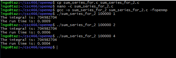
Hands-on 2: Improving sum series implementation

In the EXPLORER window, right-click on csc466/openmp and select New File.
Type sum_series_for_2.c as the file name and hits Enter.
Enter the following source code in the editor windows:
Save the file when you are done:
- Ctrl-S for Windows/Linux
- Command-S for Macs
Memorize your key-combos!.

#include <omp.h>
#include <stdio.h>
#include <stdlib.h>
#include <time.h>

int main (int argc, char *argv[]) {
  int N = atoi(argv[1]);
  int nthreads = atoi(argv[2]);
  int partial_sum[nthreads];
  clock_t start, end;

  omp_set_num_threads(nthreads);
  start = clock();
  #pragma omp parallel
  {
    int tid = omp_get_thread_num();
    partial_sum[tid] = 0;
    int psum = 0;
    #pragma omp for
    for (int i = 0; i <  N; i++) {
      psum += i;
    }
    partial_sum[tid] = psum;
  }
  end = clock();

  int sum = 0;
  for (int i = 0; i < nthreads; i++) {
    sum += partial_sum[i];
  }
  printf("The integral is: %d\n", sum);
  printf("The run time is: %.4f\n", ((double) (end - start)) / CLOCKS_PER_SEC);
  return 0;
}

compile and run sum_series_for_2.c

Key Points

Parallel for allows simplification of code

Overview

Teaching: 0 min
Exercises: 0 min

Questions

How do OpenMP threads implicitly and explicitly share work among themsleves?

How do data are managed?

Objectives

Understand the basic work sharing constructs: for, secions, and single.

Understand thread-based data sharing in OpenMP

Understand the outcomes of OpenMP programs with different work sharing constructs.

1. Work sharing constructs

OpenMP utilizes work sharing constructs to facilitate dividing parallelizable work among a number of threads.

The work sharing constructs are:

for: divide loop iterations among threads.

sections: divide sections of codes among themselves.

single: the section is executed by a single thread.

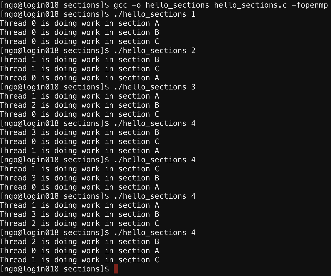
2. Work sharing construct: sections

Used when parallelize predetermined number of independent work units.

Within a primary sections construct, there can be multiple section construct.

A section can be executed by any available thread in the current team, including having multiple sections done by the same thread.

3. Hands on: sections

In the EXPLORER window, double-click on csc466/openmp and select New Dir to create a new directory in openmp called sections.

Inside sections, create a file named hello_sections.c with the following contents:

4. Challenge

Given the following functions: y=x⁴ + 15x³ + 10x² + 2x
develop an OpenMP program called poly_openmp.c with sections/section directives. Each section should handle the calculations for one term of the polynomial.

Solution

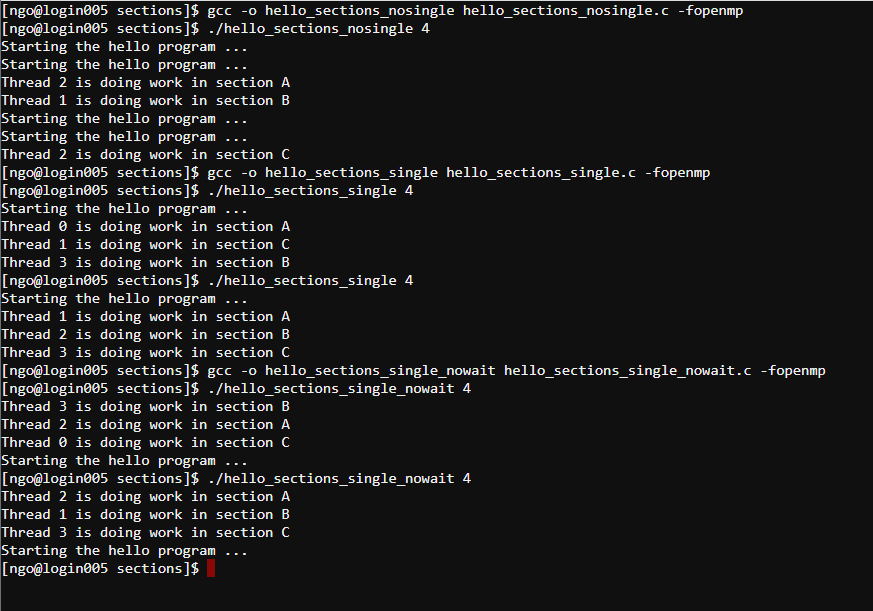
5. Work sharing construct: single

Limits the execution of a block to a single thread.

All other threads will skip the execution of this block but wait until the block is finished before moving on.

To enable proceed without waiting, a nowait clause can be added.

6. Hands on: single

Inside sections, create the following files:

hello_sections_nosingle.c:

hello_sections_single.c:

hello_sections_single_nowait.c:

Compile and run the above files:

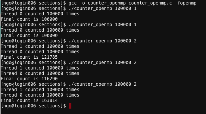
7. Shared and private data

Data declared outside of a parallel region will be shared among all threads.

Data declared inside of a parallel region will be private to individual thread.

8. Hands on: problem with shared data

Inside sections, create a file named counter_openmp.c with the following contents:

Key Points

Introduction to MPI

Overview

Teaching: 0 min
Exercises: 0 min

Questions

Objectives

Understand the origin of message passing interface (MPI)

Know the basic MPI routines to identify rank and get total number of participating processes.

Understand how to leverage process rank and total process count for work assignment.

1. Message passing

Processes communicate via messages

Messages can be:

Raw data used in actual calculations

Signals and acknowledgements for the receiving processes regarding the workflow.

2. History of MPI: early 80s

Various message passing environments were developed.

Many similar fundamental concepts:

Cosmic Cube and nCUBE/2 (Caltech),

P4 (Argonne),

PICL and PVM (Oakridge),

LAM (Ohio SC)

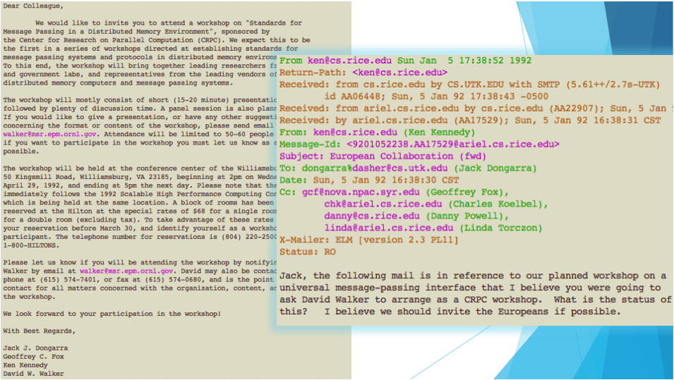
3. History of MPI: 1991-1992

More than 80 researchers from different institutions in US and Europe agreed to develop and implement a common standard for message passing.

Follow-up first meeting of the working group hosted at Supercomputing 1992 in Minnesota.

4. After finalization of working technical draft

MPI becomes the de-facto standard for distributed memory parallel programming.

Available on every popular operating system and architecture.

Interconnect manufacturers commonly provide MPI implementations optimized for their hardware.

MPI standard defines interfaces for C, C++, and Fortran.

Language bindings available for many popular languages (quality varies)

Python (mpi4py)

Java (no longer active)

5. 1994: MPI-1

Communicators

Information about the runtime environments

Creation of customized topologies

Point-to-point communication

Send and receive messages

Blocking and non-blocking variations

Collectives

Broadcast and reduce

Gather and scatter

6. 1998: MPI-2

One-sided communication (non-blocking)

Get & Put (remote memory access)

Dynamic process management

Spawn

Parallel I/O

Multiple readers and writers for a single file

Requires file-system level support (LustreFS, PVFS)

7. 2012: MPI-3

Revised remote-memory access semantic

Fault tolerance model

Non-blocking collective communication

Access to internal variables, states, and counters for performance evaluation purposes

8. Hands-on: taz and submitty

Your account (login/password) will work on both taz and submitty.

USERNAME represents the login name that you received in email.

To access taz from a terminal:
$ ssh USERNAME@taz.cs.wcupa.edu
To access submitty from a terminal:
$ ssh USERNAME@submitty.cs.wcupa.edu
The environments on taz and submitty are similar to one another. In the remainder of these lectures, example screenshots will be taken from submitty, but all commands will work on taz as well.

9. Hands-on: create and compile MPI codes

Create a directory named intro-mpi

Change into intro-mpi
$ cd
$ mkdir intro-mpi
$ cd intro-mpi
To create a file from terminal, run nano -c file_name.

When finish editing, press Ctrl-X to select Quit and Save.

Press Y to confirm that you want to save.

Press Enter to confirm that you are saving to file_name.

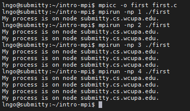
Inside intro-mpi, create a file named first.c with the following contents

Compile and run first.c:
$ mpicc -o first first.c
$ mpirun -np 1 ./first
$ mpirun -np 2 ./first
$ mpirun -np 4 ./first
Both taz and submitty only have four computing cores, therefore we can (should) only run to a maximum of four processes.

10. MPI in a nutshell

All processes are launched at the beginning of the program execution.

The number of processes are user-specified

This number could be modified during runtime (MPI-2 standards)

Typically, this number is matched to the total number of cores available across the entire cluster

All processes have their own memory space and have access to the same source codes.

MPI_Init: indicates that all processes are now working in message-passing mode.

MPI_Finalize: indicates that all processes are now working in sequential mode (only one process active) and there are no more message-passing activities.

11. MPI in a nutshell

MPI_COMM_WORLD: Global communicator

MPI_Comm_rank: return the rank of the calling process

MPI_Comm_size: return the total number of processes that are part of the specified communicator.

MPI_Get_processor_name: return the name of the processor (core) running the process.

12. MPI communicators (first defined in MPI-1)

MPI defines communicator groups for point-to-point and collective communications:

Unique IDs (rank) are defined for individual processes within a communicator group.

Communications are performed based on these IDs.

Default global communication (MPI_COMM_WORLD) contains all processes.

For N processes, ranks go from 0 to N−1.

13. Hands-on: hello.c

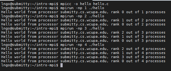
Inside intro-mpi, create a file named hello.c with the following contents

Compile and run hello.c:
$ mpicc -o hello hello.c
$ mpirun -np 1 ./hello
$ mpirun -np 2 ./hello
$ mpirun -np 4 ./hello

14. Hands-on: evenodd.c

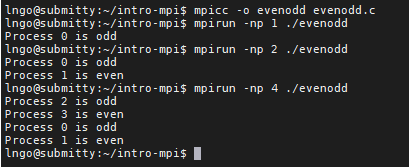
In MPI, processes’ ranks are used to enforce execution/exclusion of code segments within the original source code.

Inside intro-mpi, create a file named evenodd.c with the following contents

Compile and run evenodd.c:
$ mpicc -o evenodd evenodd.c
$ mpirun -np 1 ./evenodd
$ mpirun -np 2 ./evenodd
$ mpirun -np 4 ./evenodd

15. Hands-on: rank_size.c

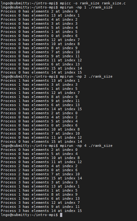
In MPI, the values of ranks and size can be used as means to calculate and distribute workload (data) among the processes.

Inside intro-mpi, create a file named rank_size.c with the following contents

Compile and run rank_size.c:
$ mpicc -o rank_size rank_size.c
$ mpirun -np 1 ./rank_size
$ mpirun -np 2 ./rank_size
$ mpirun -np 4 ./rank_size

Key Points

MPI: point-to-point, data types, and communicators

Overview

Teaching: 0 min
Exercises: 0 min

Questions

How can processes pass messages directly to one another (point-to-point)

Objectives

Understand meaning of parameters in syntax of MPI_Send and MPI_Recv

Understand the proper ordering of p2p communication to avoid deadlock.

Know how to invoke MPI_Send and MPI_Recv to transfer data between processes.

1. Addresses in MPI

Data messages (objects) being sent/received (passed around) in MPI are referred to by their addresses:

Memory location to read from to send

Memory location to write to after receiving.

2. Parallel workflow

Individual processes rely on communication (message passing) to enforce workflow

Point-to-point communication: MPI_Send, MPI_Recv

Collective communication: MPI_Broadcast, MPI_Scatter, MPI_Gather, MPI_Reduce, MPI_Barrier.

3. Point-to-point: MPI_Send and MPI_Recv

int MPI_Send(void *buf, int count, MPI_Datatype datatype, int dest, int tag, MPI_Comm comm)

*buf: pointer to the address containing the data elements to be sent.

count: how many data elements will be sent.

MPI_Datatype: MPI_BYTE, MPI_PACKED, MPI_CHAR, MPI_SHORT, MPI_INT, MPI_LONG, MPI_FLOAT, MPI_DOUBLE, MPI_LONG_DOUBLE, MPI_UNSIGNED_CHAR, and other user-defined types.

dest: rank of the process these data elements are sent to.

tag: an integer identify the message. Programmer is responsible for managing tag.

comm: communicator (typically just used MPI_COMM_WORLD)

int MPI_Recv(void *buf, int count, MPI_Datatype datatype, int source, int tag, MPI_Comm comm, MPI_Status *status)

*buf: pointer to the address containing the data elements to be written to.

count: how many data elements will be received.

MPI_Datatype: MPI_BYTE, MPI_PACKED, MPI_CHAR, MPI_SHORT, MPI_INT, MPI_LONG, MPI_FLOAT, MPI_DOUBLE, MPI_LONG_DOUBLE, MPI_UNSIGNED_CHAR, and other user-defined types.

dest: rank of the process from which the data elements to be received.

tag: an integer identify the message. Programmer is responsible for managing tag.

comm: communicator (typically just used MPI_COMM_WORLD)

*status: pointer to an address containing a special MPI_Status struct that carries additional information about the send/receive process.

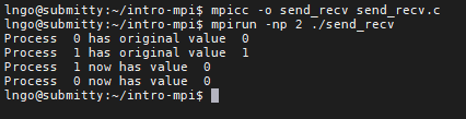
4. Hands-on: send_recv.c

We want to write a program called send_recv.c that allows two processes to exchange their ranks:

Process 0 receives 1 from process 1.

Process 1 receives 0 from process 0.

Inside intro-mpi, create a file named send_recv.c with the following contents

Compile and run send_recv.c:
$ mpicc -o send_recv send_recv.c
$ mpirun -np 2 ./send_recv
Did we get what we want? Why?

Correction: separate sending and receiving buffers.

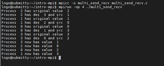
5. Hands-on: p2p communication at scale

Rely on rank and size and math.

We want to shift the data elements with only message passing among adjacent processes.

Inside intro-mpi, create a file named multi_send_recv.c with the following contents

Compile and run multi_send_recv.c:
$ mpicc -o multi_send_recv multi_send_recv.c
$ mpirun -np 4 ./multi_send_recv
Did we get what we want? Why?

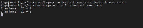
6. Hands-on: blocking risk

MPI_Recv is a blocking call.

Meaning the process will stop until it receives the message.

What if the message never arrives?

Inside intro-mpi, create a file named deadlock_send_recv.c with the following contents

Compile and run deadlock_send_recv.c:
$ mpicc -o deadlock_send_recv deadlock_send_recv.c
$ mpirun -np 2 ./deadlock_send_recv
What happens?

To get out of deadlock, press Ctrl-C.

Correction:

Pay attention to send/receive pairs.

The numbers of MPI_Send must always equal to the number of MPI_Recv.

MPI_Send should be called first (preferably).

Key Points

MPI: Functional parallelism and collectives

Overview

Teaching: 0 min
Exercises: 0 min

Questions

How do multiple processes communicate as a group at the same time?

Objectives

Understand how collective communication work relative to process ranking.

Know how to properly invoke a collective MPI routine to carry out a data distribution/collection/reduction task.

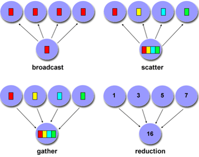
1. Collective communication

Must involve ALL processes within the scope of a communicator.

Unexpected behavior, including programming failure, if even one process does not participate.

Types of collective communications:

Synchronization: barrier

Data movement: broadcast, scatter/gather

Collective computation (aggregate data to perform computation): Reduce

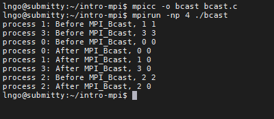
2. Hands-on: MPI_Bcast

int MPI_Bcast(void *buf, int count, MPI_Datatype datatype, int root, MPI_Comm comm)

*buf:

If on root, pointer to the address containing the data elements to be broadcasted

If not on root, pointer to the address where broadcasted data to be stored.

count: how many data elements will be broadcasted.

MPI_Datatype: MPI_BYTE, MPI_PACKED, MPI_CHAR, MPI_SHORT, MPI_INT, MPI_LONG, MPI_FLOAT, MPI_DOUBLE, MPI_LONG_DOUBLE, MPI_UNSIGNED_CHAR, and other user-defined types.

root: rank of the process where the original data will be broadcasted.

tag: an integer identify the message. Programmer is responsible for managing tag.

comm: communicator (typically just used MPI_COMM_WORLD)

Don’t need to specify a TAG or DESTINATION

Must specify the SENDER (root)

Blocking call for all processes

Inside intro-mpi, create a file named bcast.c with the following contents

Compile and run bcast.c:
$ mpicc -o bcast bcast.c
$ mpirun -np 4 ./bcast

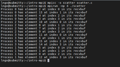
3. Hands-on: MPI_Scatter

int MPI_Scatter(void *sendbuf, int sendcount, MPI_Datatype sendtype, void *recvbuf,int recvcount,MPI_Datatype recvtype, int root, MPI_Comm comm)

*sendbuf: pointer to the address containing the array of data elements to be scattered.

sendcount: how many data elements to be sent to each process of the communicator.

*recvbuf: pointer to the address on each process of the communicator, where the scattered portion will be written.

recvcount: how many data elements to be received by each process of the communicator.

root: rank of the process from where the original data will be scattered.

comm: communicator (typically just used MPI_COMM_WORLD)

Inside intro-mpi, create a file named scatter.c with the following contents

Compile and run scatter.c:
$ mpicc -o scatter scatter.c
$ mpirun -np 4 ./scatter

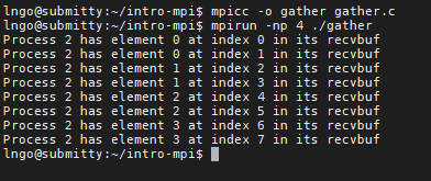
4. Hands-on: MPI_Gather

int MPI_Gather(void *sendbuf, int sendcount, MPI_Datatype sendtype, void *recvbuf,int recvcount,MPI_Datatype recvtype, int root, MPI_Comm comm)

*sendbuf: pointer to the address on each process of the communicator, containing the array of data elements to be gathered.

sendcount: how many data elements from each process of the communicator to be sent back to the root process.

*recvbuf: pointer to the address on the root process where all gathered data will be written.

recvcount: how many data elements to be received from each process of the communicator.

root: rank of the process from where the original data will be gathered.

comm: communicator (typically just used MPI_COMM_WORLD)

Inside intro-mpi, create a file named gather.c with the following contents

Compile and run gather.c:
$ mpicc -o gather gather.c
$ mpirun -np 4 ./gather

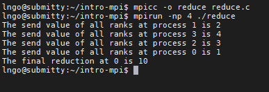
5. Hands-on: MPI_Reduce

int MPI_Reduce(void *sendbuf, void *recvbuf, int count, MPI_Datatype datatype, MPI_OP op,int root, MPI_Comm comm)

*sendbuf: pointer to the address on each process of the communicator, containing the array of data elements to be reduced.

*recvbuf: pointer to the address on the root process where all final reduced data will be written.

count: how many data elements to be received from each process of the communicator. If count > 1, then operation is performed element-wise.

op: may be MPI_MIN, MPI_MAX, MPI_SUM, MPI_PROD (twelve total). Programmer may add operations, must be commutative and associative.

root: rank of the process from where the original data will be gathered.

comm: communicator (typically just used MPI_COMM_WORLD).

Inside intro-mpi, create a file named gather.c with the following contents

Compile and run reduce.c:
$ mpicc -o reduce reduce.c
$ mpirun -np 4 ./reduce

Key Points

MPI: pleasantly parallel and workload allocation

Overview

Teaching: 0 min
Exercises: 0 min

Questions

Objectives

Understand the characteristics that make a computational job pleasantly parallel.

Know the various approach to workload division in pleasantly parallel.

1. Definition

Embarrassingly/naturally/pleasantly parallel.

A computation that can obviously be divided into a number of completely different parts, each of which can be executed by a separate process.

Each process can do its tasks without any interaction with the other processes, therefore, …

No communication or very little communication among the processes.

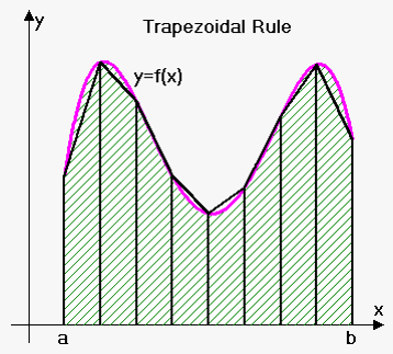
2. Example: integral estimation using the trapezoid method

A technique to approximate the integral of a function f.

Integral is defined as the area of the region bounded by the graph f, the x-axis, and two vertical lines x=a and x=b.

We can estimate this area by dividing it into infinitesimal trapezoids.

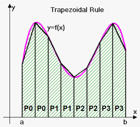
3. Example: integral estimation using the trapezoid method

Divide the area under the curve into 8 trapezoids with equal base h.

N = 8

a = 0

b = 2

The base h can be calculated as:

h = (b - a) / N = 0.25

4. Example: integral estimation using the trapezoid method

Which trapezoid (workload/task) goes to which process?

Start with small number of processes.

Calculation workload assignment manually for each count of processes.

Generalize assignment for process i based on sample calculations.

5. Example: integral estimation using the trapezoid method

4 processes: P0, P1, P2, P3: size = 4

N = 8

a = 0

b = 2

The height h can be calculated as:

h = (b - a) / N = 0.25

The amount of trapezoid per process:

local_n = N / size = 2;

local_a: variable represent the starting point of the local interval for each process. Variable local_a will change as processes finish calculating one trapezoid and moving to another.

local_a for P0= 0 = 0 + 0 * 2 * 0.25

local_a for P1= 0.5 = 0 + 1 * 2 * 0.25

local_a for P2= 1 = 0 + 2 * 2 * 0.25

local_a for P2= 1.5 = 0 + 3 * 2 * 0.25

6. Handson: integral estimation using the trapezoid method

Your account (login/password) will work on both taz and submitty.

USERNAME represents the login name that you received in email.

To access taz from a terminal:
$ ssh USERNAME@taz.cs.wcupa.edu
To access submitty from a terminal:
$ ssh USERNAME@submitty.cs.wcupa.edu
The environments on taz and submitty are similar to one another. In the remainder of these lectures, example screenshots will be taken from submitty, but all commands will work on taz as well.

Change into intro-mpi
$ cd intro-mpi
To create a file from terminal, run nano -c file_name.

When finish editing, press Ctrl-X to select Quit and Save.

Press Y to confirm that you want to save.

Press Enter to confirm that you are saving to file_name.

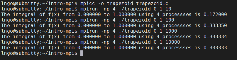
Inside intro-mpi, create a file named trapezoid.c with the following contents

Compile and run trapezoid.c:
$ mpicc -o trapezoid trapezoid.c
$ mpirun -np 4 ./trapezoid 0 1 10
$ mpirun -np 4 ./trapezoid 0 1 100
$ mpirun -np 4 ./trapezoid 0 1 1000
$ mpirun -np 4 ./trapezoid 0 1 10000

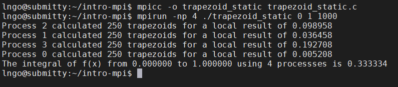
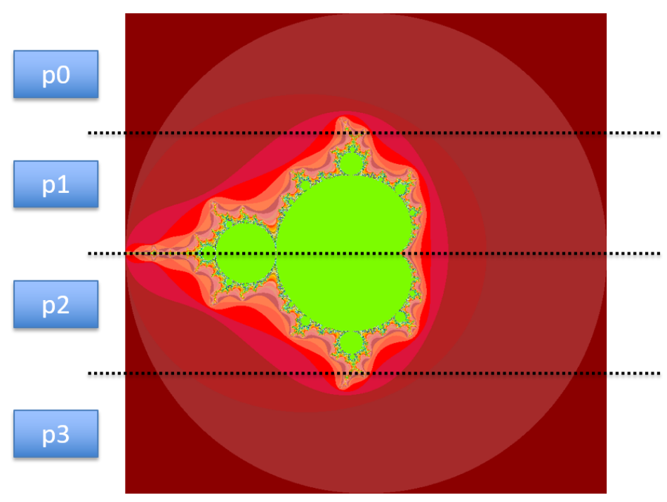
7. Hands-on: static workload assignment

Is this fair?

Create a copy of trapezoid.c called trapezoid_static.c and modify trapezoid_static.c to have the following contents

Compile and run trapezoid_static.c:
$ mpicc -o trapezoid_static trapezoid_static.c
$ mpirun -np 4 ./trapezoid_static 0 1 1000
This is called static workload assignment.

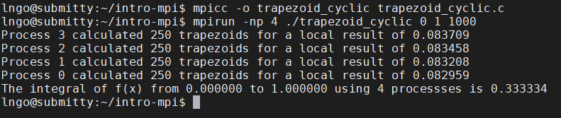
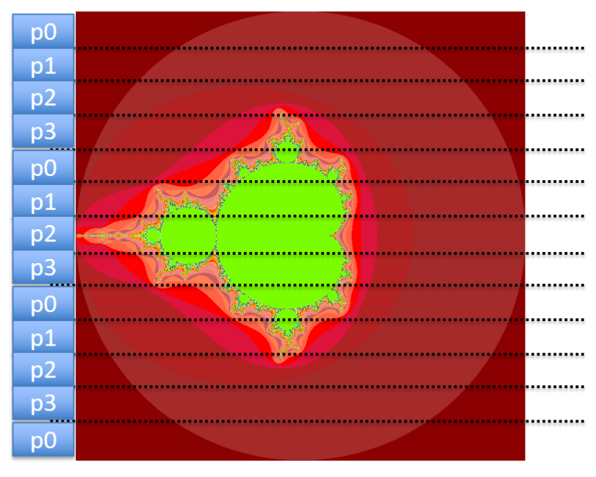
8. Hands-on: cyclic workload assignment

Create a copy of trapezoid_static.c called trapezoid_cyclic.c and modify trapezoid_cyclic.c to have the following contents

Compile and run trapezoid_cyclic.c:
$ mpicc -o trapezoid_cyclic trapezoid_cyclic.c
$ mpirun -np 4 ./trapezoid_cyclic 0 1 1000
This is called cyclic workload assignment.

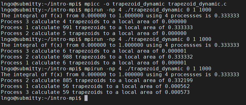
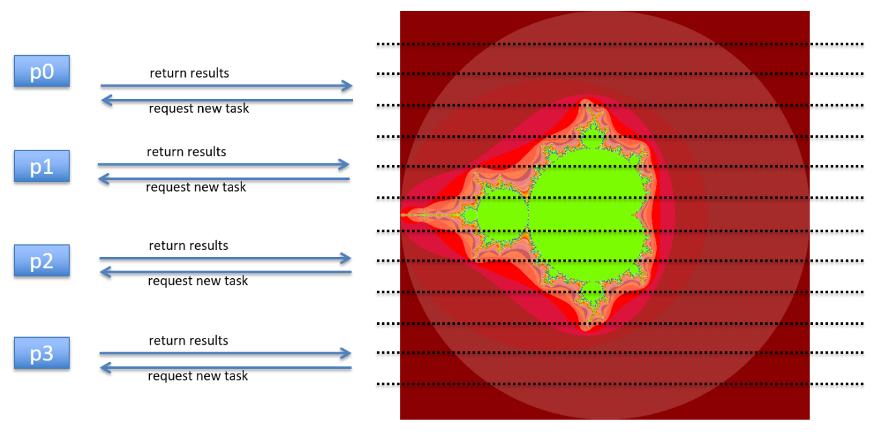
9. Hands-on: dynamic workload assignment

Create a file called trapezoid_dynamic_.c with the following contents:

Compile and run trapezoid_dynamic.c:
$ mpicc -o trapezoid_dynamic trapezoid_dynamic.c
$ mpirun -np 4 ./trapezoid_dynamic 0 1 1000
$ mpirun -np 4 ./trapezoid_dynamic 0 1 1000
$ mpirun -np 4 ./trapezoid_dynamic 0 1 1000
This is called dynamic workload assignment.

Key Points

Introduction to CloudLab

Overview

Teaching: 0 min
Exercises: 0 min

Questions

Objectives

1. What is CloudLab

Experimental testbed for future computing research

Allow researchers control to the bare metal

Diverse, distributed resources at large scale

Allow repeatable and scientific design of experiments

2. What is GENI

Global Environment for Networking Innovation

Combining heterogeneous resource types, each virtualized along one or more suitable dimensions, to produce a single platform for network science researchers”

Key components:

GENI racks: virtualized computation and storage resources

Software-defined networks (SDNs): virtualized, programmable network resources

WiMAX: virtualized cellular wireless communication

Berman, M., Chase, J.S., Landweber, L., Nakao, A., Ott, M., Raychaudhuri, D., Ricci, R. , and Seskar, I., 2014. GENI: A federated testbed for innovative network experiments. Computer Networks, 61, pp.5-23.

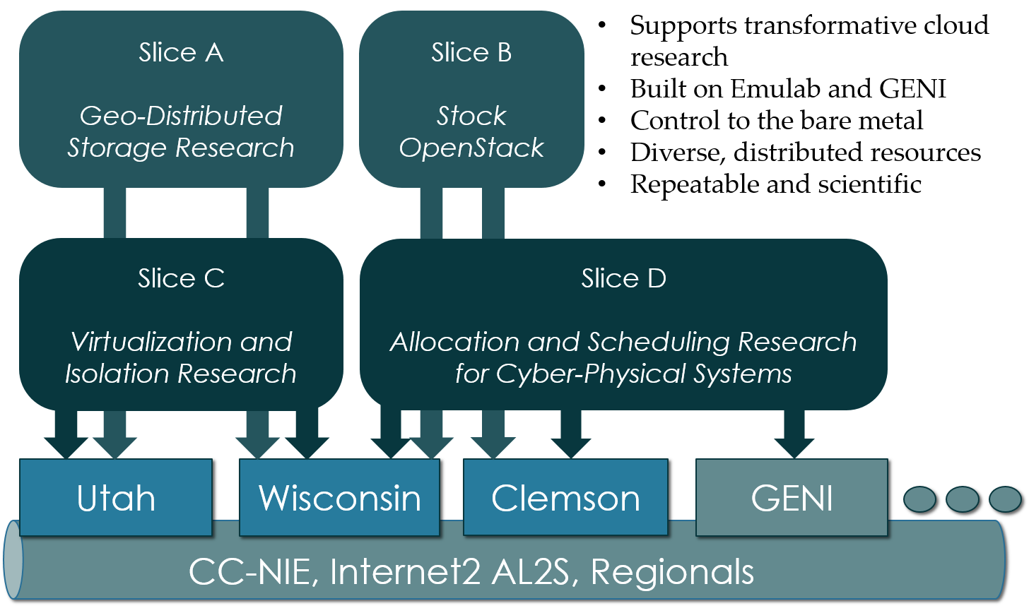
3. Key experimental concepts

Sliceability: the ability to support virtualization while maintaining some degree of isolation for simultaneous experiments

Deep programmability: the ability to influence the behavior of computing, storage, routing, and forwarding components deep inside the network, not just at or near the network edge.

4. Hardware

Utah/HP: Low-power ARM64 (785 nodes)

315 m400: 1X 8-core ARMv8 at 2.4GHz, 64GB RAM, 120GB flash

270 m510: 1X 8-core Intel Xeon D-1548 at 2.0 GHz, 64GB RAM, 256 GB flash

200 xl170: 1X 10-core Intel E5-2640v4 at 2.4 Ghz, 64 GB RAM, 480 GB SSD

Wisconsin/Cisco: 530 nodes

90 c220g1: 2X 8-core Intel Haswell at 2.4GHz, 128GB RAM, 1X 480GB SDD, 2X 1.2TB HDD

10 c240g1: 2X 8-core Intel Haswell at 2.4GHz, 128GB RAM, 1X 480GB SDD, 1X 1TB HDD, 12X 3TB HDD

163 c220g2: 2X 10-core Intel Haswell at 2.6GHz, 160GB RAM, 1X 480GB SDD, 2X 1.2TB HDD

7 c240g2: 2X Intel Haswell 10-core at 2.6GHz, 160GB RAM, 2X 480GB SDD, 12X 3TB HDD

224 c220g5: 2X 10-core Intel Skylake at 2.20GHz, 192GB RAM, 1TB HDD

32 c240g5: 2X 10-core Intel Skylake at 2.20GHz, 192GB RAM, 1TB HDD, 1 NVIDIA P100 GPU

4 c4130: 2X 8-core Intel Broadwell at 3.20GHz, 128GB RAM, 2X 960GB HDD, 4 NVIDIA V100 GPU

Clemson/Dell: 256 nodes

96 c8220: 2X 10-core Intel Ivy Bridge at 2.2GHz, 256GB RAM, 2X 1TB HDD

4 c8220x: 2X 10-core Intel Ivy Bridge at 2.2GHz, 256GB RAM, 8X 1TB HDD, 12X 4TB HDD

84 c6420: 2X 14-core Intel Haswell at 2.0GHz, 256GB RAM, 2X 1TB HDD

2 c4130: 2X 12-core Intel Haswell at 2.5GHz, 256GB RAM, 2X 1TB HDD, 2 NVIDIA K40m GPU

2 dss7500: 2X 6-core Intel Haswell at 2.4GHZ, 128GN RAM, 2X 126GB SSD, 45X 6TB HDD

72 c6420: 2X 16-core Intel Skylake at 2.6GHZ, 386GB RAM, 2X 1TB HDD

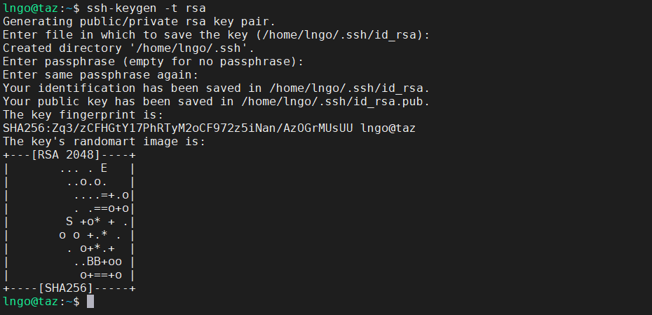
5. Setup SSH

SSH into taz.cs.wcupa.edu or submitty.cs.wcupa.edu and run the following commands:

Hit Enter for all questions. Do not enter a password or change the default location of the files.
$ cd
$ ssh-keygen -t rsa
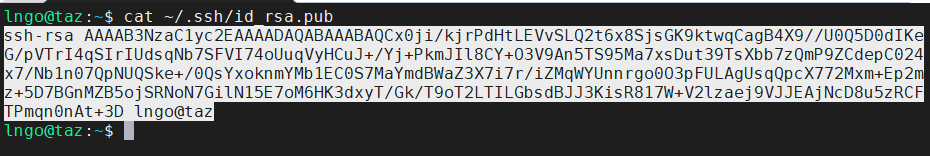
Run the following command to display the public key

Drag your mouse over to paint/copy the key (just the text, no extra spaces after the last character)
$ cat ~/.ssh/id_rsa.pub
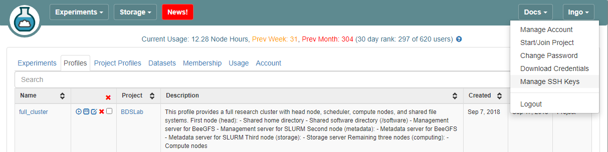
Log into CloudLab, click on your username (top right) and select Manage SSH Keys:

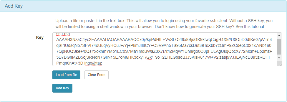
Paste the key into the Key box and click Add Key:

6. Setup GitHub repository

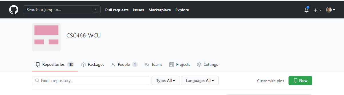
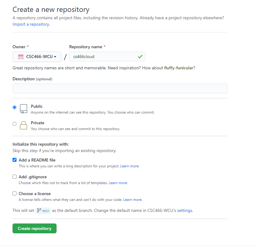
Go to your GitHub account, under Repositories, select New.

You can select any name for your repo.

It must be public.

The Add a README file box must be checked.

Click Create repository when done.

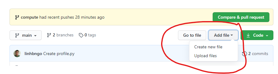
Click Add file and select Create new file

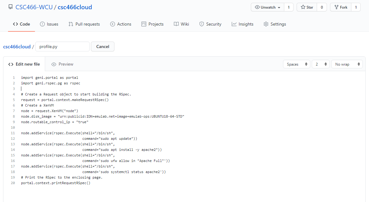
Type profile.py for the file name and enter THIS CONTENT into the text editor.

Click Commit new file when done.

7. Setup CloudLab profile

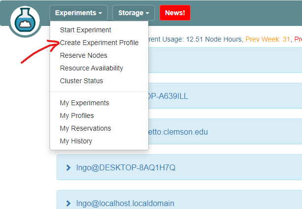
Login to your CloudLab account, click Experiments on top left, select Create Experiment Profile.

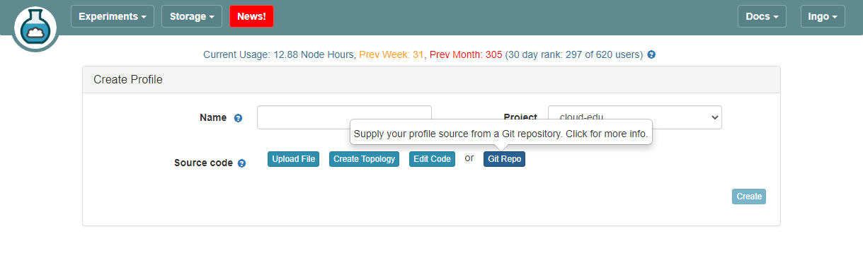
Click on Git Repo

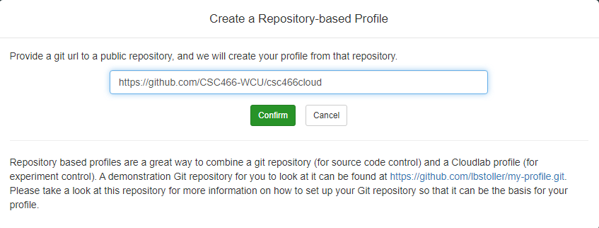
Paste the URL of your previously created Git repo here and click Confirm

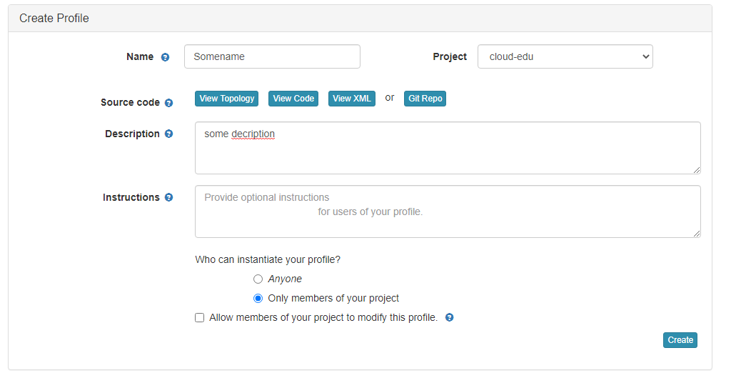
Enter the name for your profile, put in some words for the Description.

You will not have a drop-down list of Project.

Click Create when done.

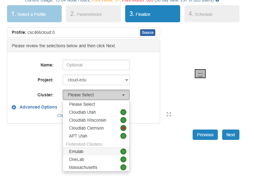
Click Instantiate to launch an experiment from your profile.

Select a Cluster from Wisconsin, Clemson, or Emulab, then click Next.

Do not do anything on the next Start on date/time screen. Click Finish.

Your experiment is now being provision, and then `booting

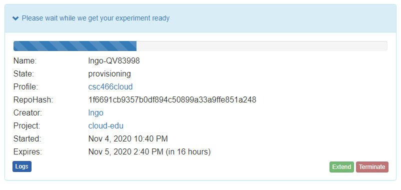
When it is ready, you can use the provided SSH command to log in to your experiment (assuming your key was set up correctly)

Key Points

Deploying compute nodes for a supercomputer

Overview

Teaching: 0 min
Exercises: 0 min

Questions

How do we deploy compute nodes and relevant software programmatically?

Objectives

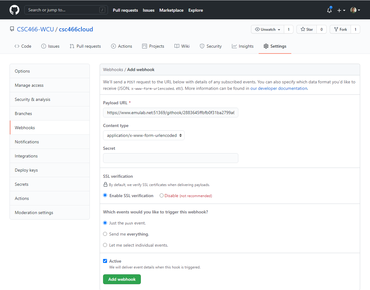
1. Setup webhook in CloudLab

Webhook is a mechanism to automatically push any update on your GitHub repo to the corresponding CloudLab repository.

Login to CloudLab.

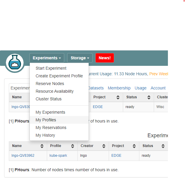
Top left, under Experiments, select My Profiles.

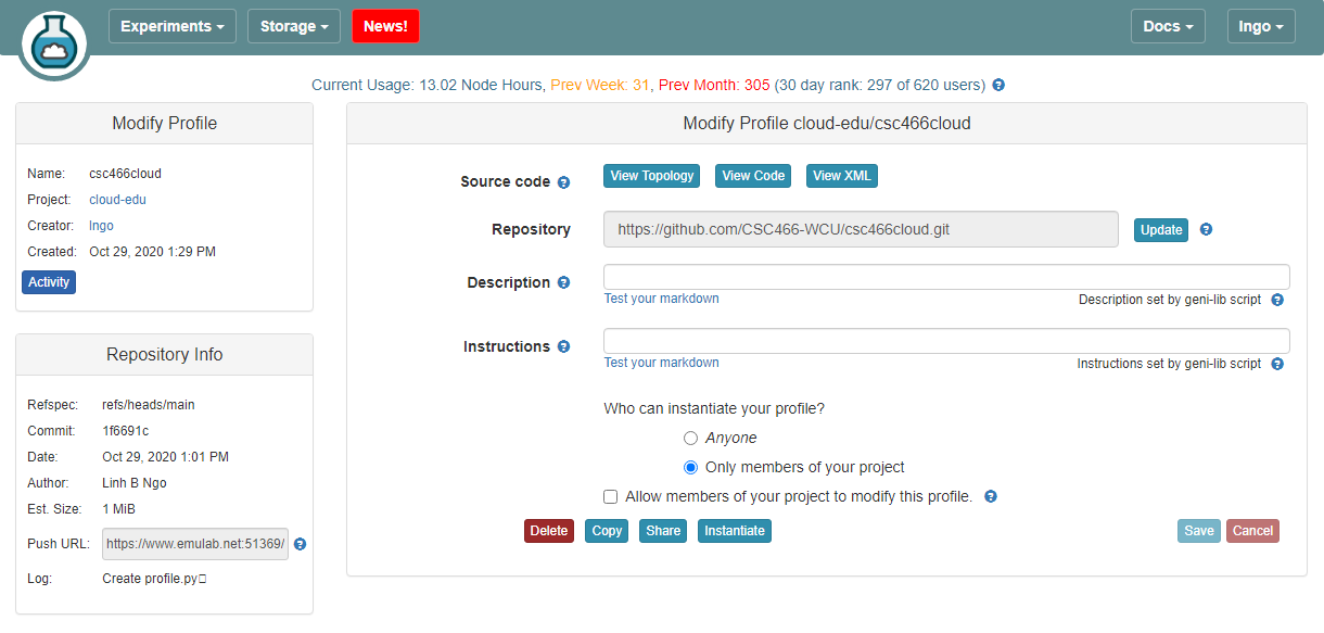
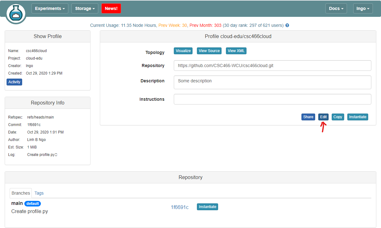
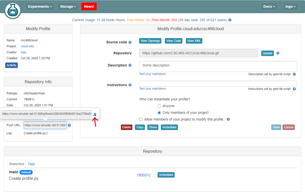
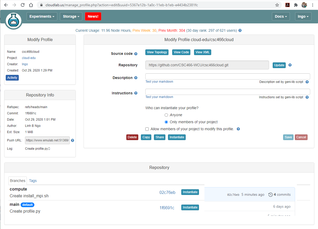
Click on the profile created for CSC466, then select Edit

Click on the Push URL bar, then click on the blue Clipboard icon.

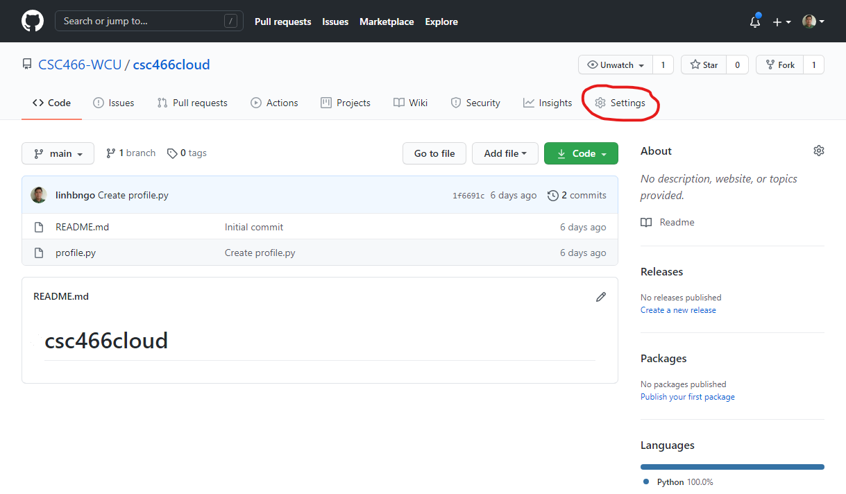
Go to the corresponding GitJub repository and go to Settings.

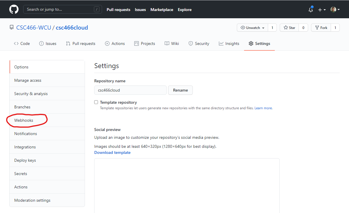
Go to Webhooks.

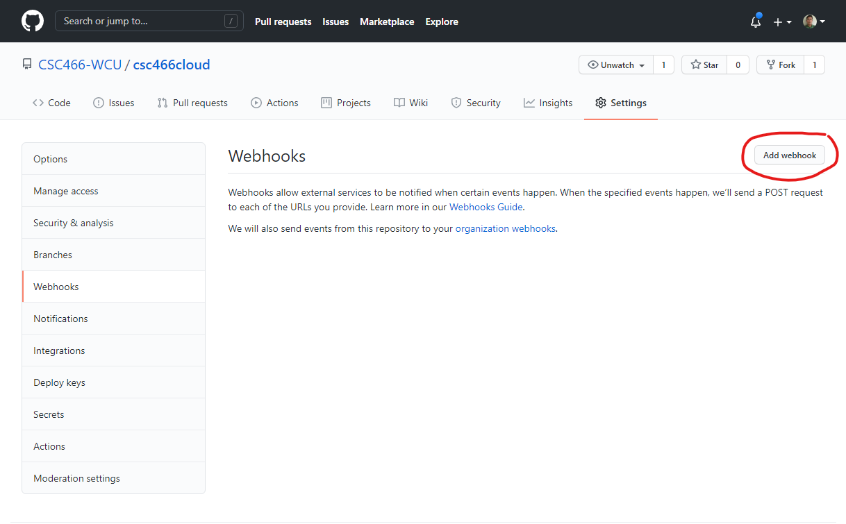
Click Add webhook. You will need to re-enter the password for your GitHub account next.

Pass the value copied from the clipboard in CloudLab into the Payload URL box.

Click on Add webhook.

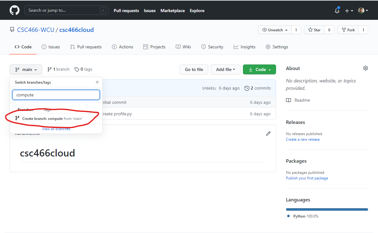
2. Create a new branch on your GitHub repo

In your GitHub repository, create a new branch called compute.

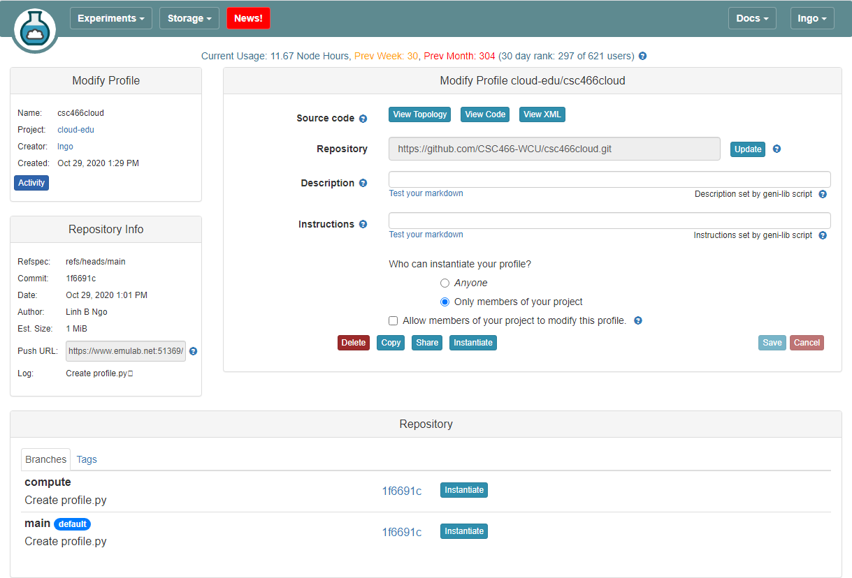
If you set up your webhook correctly, compute should show up on your CloudLab profile as well

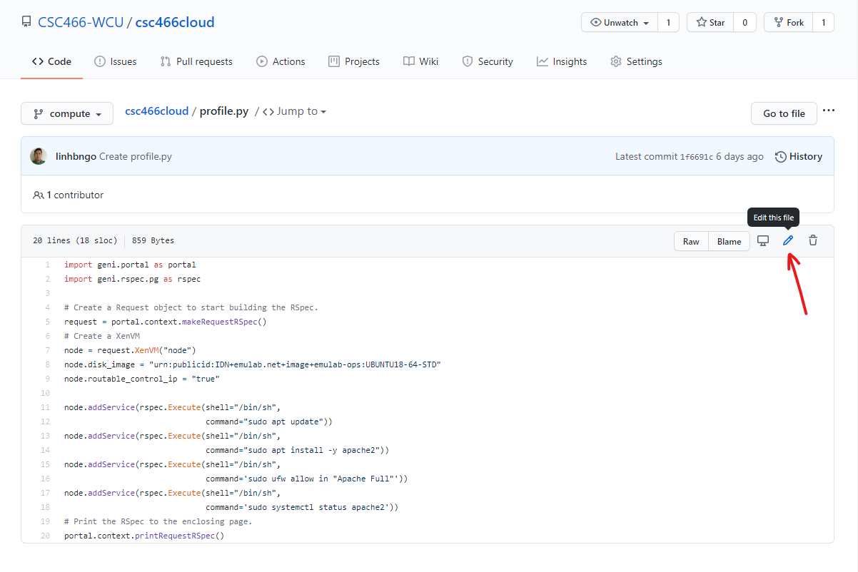
In your GitHub repository, edit the profile.py file with THIS CONTENT.

Click Commit changes once done to save.

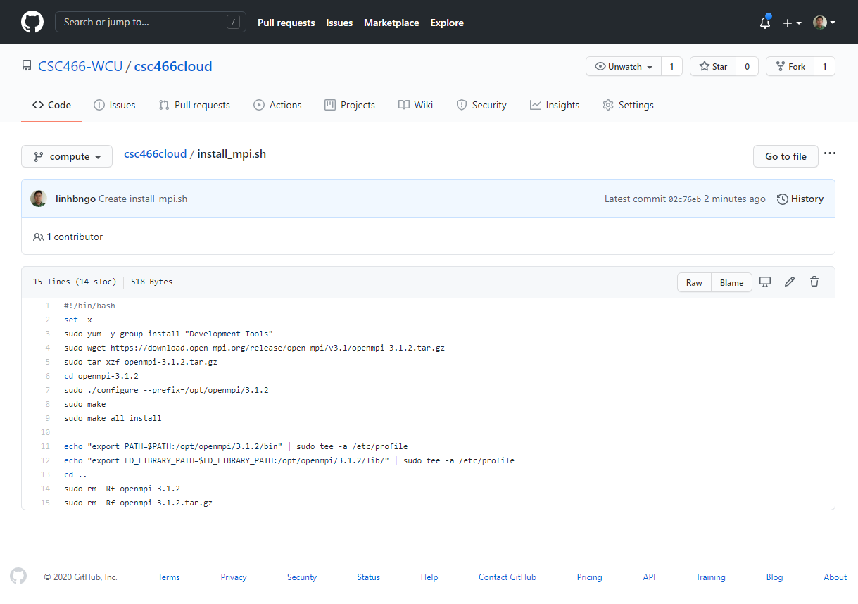
Create a new file called install_mpi.sh with THIS CONTENT

Click Commit new file once done to save.

Go to CloudLab, refresh the page, and confirm that the hash of your compute branch here match with the hash on GitHub repo.

Instantiate from the compute branch.

Key Points

Distributed File Systems

Overview

Teaching: 0 min
Exercises: 0 min

Questions

How to arrange read/write accesses with processes running on computers that are part of a computing cluster?

Objectives

0. Hands-on: What does it take to run MPI on a distributed computing system?

Log into CloudLab

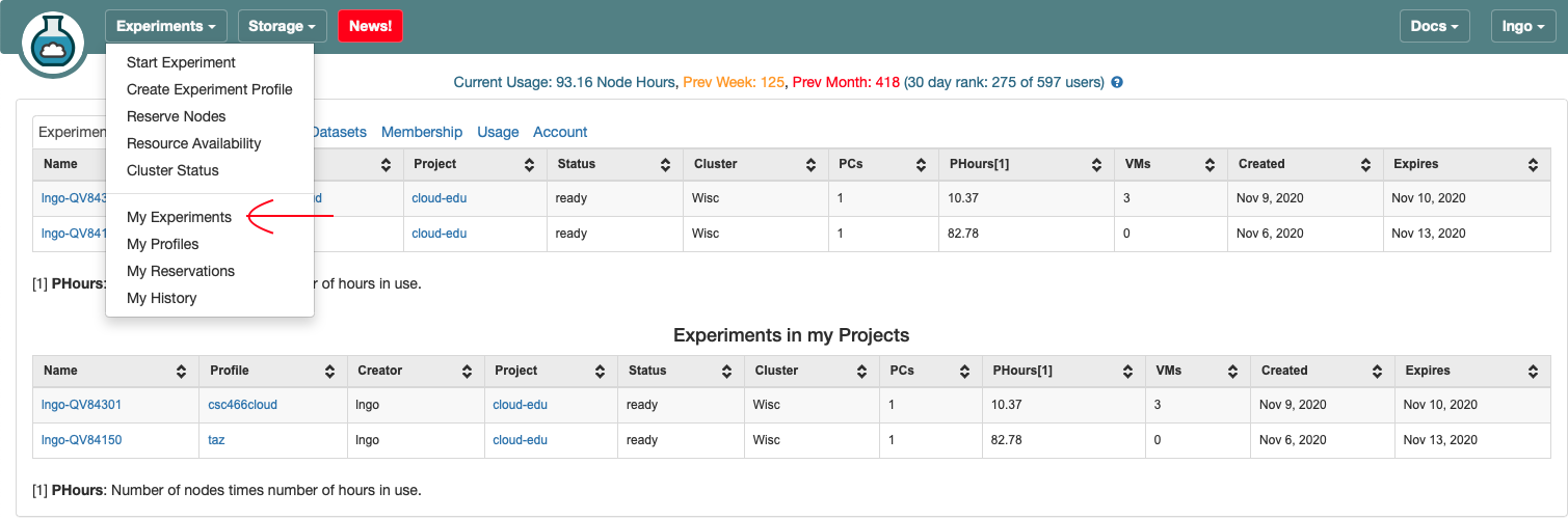
Go to Experiments/My Experiments

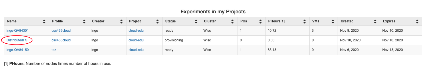
Go to the DistributedFS experiment under Experiments in my Projects.

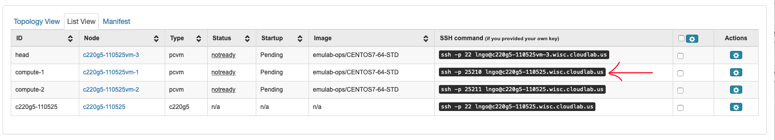
Under the List View tab, SSH command column, use the provided SSH command to login to compute-1.

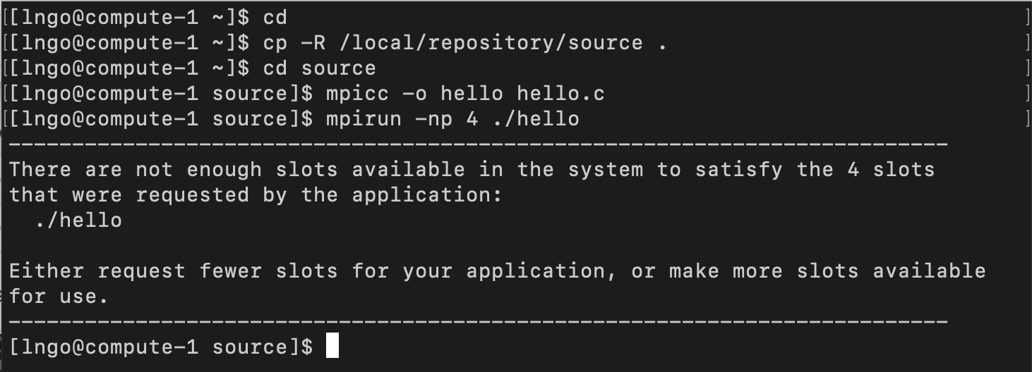
Run the following bash commands from your home directory:
$ cd
$ cp -R /local/repository/source .
$ cd source
$ mpicc -o hello hello.c 
$ mpirun -np 4 ./hello
What does it take to run on multiple cores?

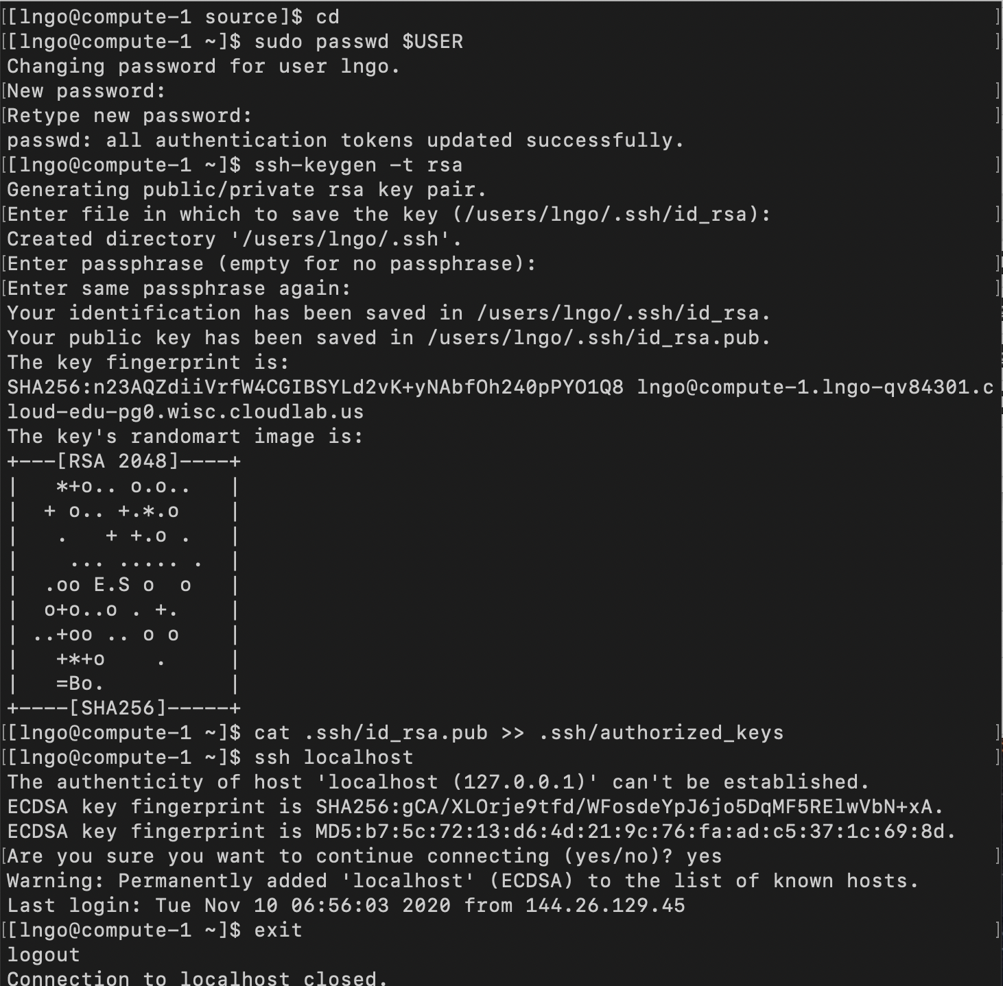
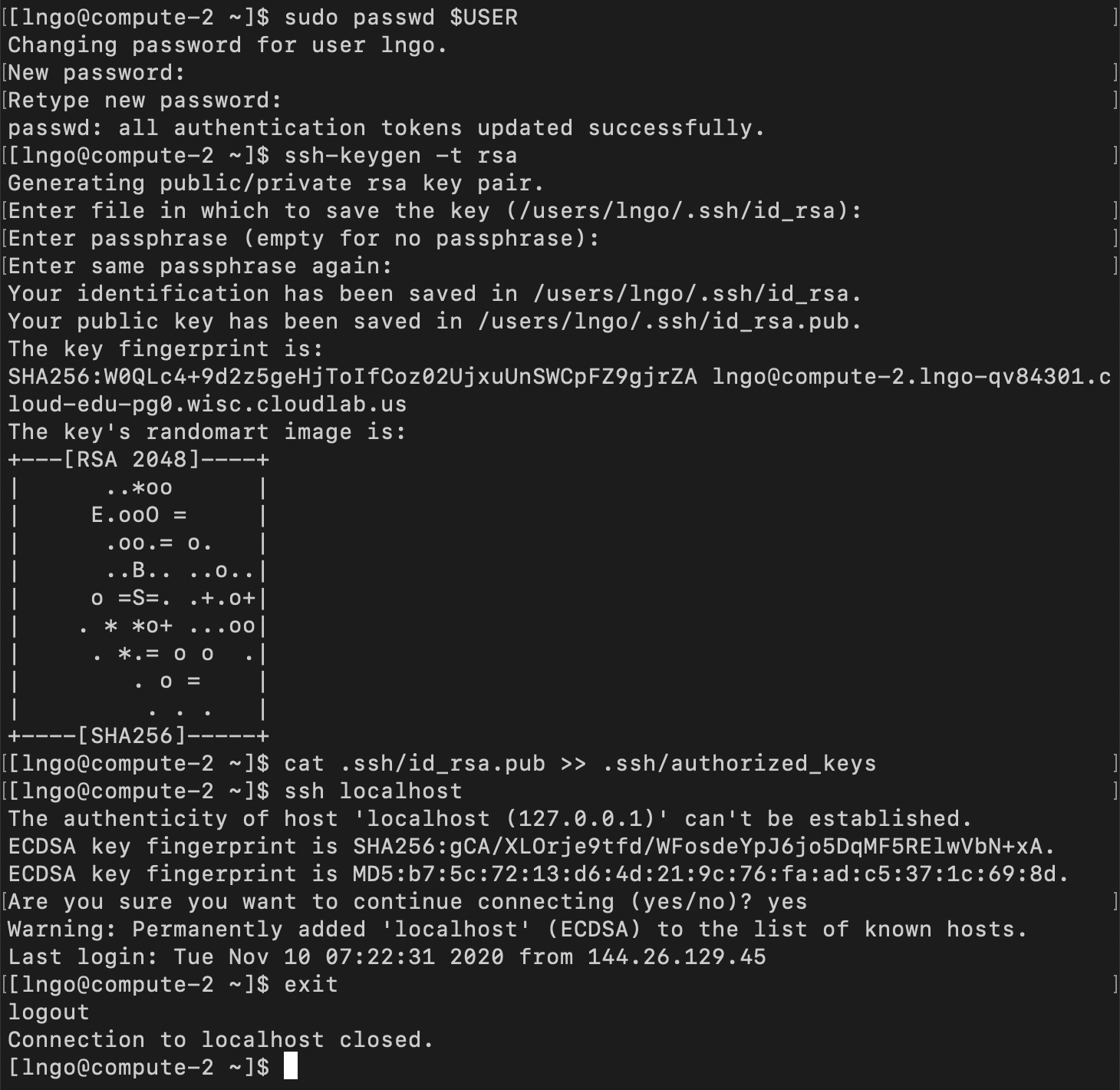
MPI runs on SSH: needs to setup passwordless SSH (hit Enter across all questions!)

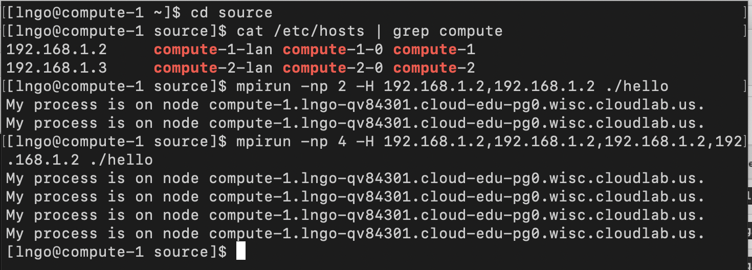
Needs to specify IP addresses for each core on host.
$ cd 
$ sudo passwd $USER
$ ssh-keygen -t rsa
$ cat .ssh/id_rsa.pub >> .ssh/authorized_keys
$ ssh localhost
$ exit
$ cd source
$ cat /etc/hosts | grep compute
$ mpirun -np 2 -H 192.168.1.2,192.168.1.2 ./hello
$ mpirun -np 4 -H 192.168.1.2,192.168.1.2,192.168.1.2,192.168.1.2 ./hello
How can we get this to run across multiple nodes?

Open a new terminal.

Log into compute-2 and repeat the above process to create password and passwordless SSH.
$ cd 
$ sudo passwd $USER
$ ssh-keygen -t rsa
$ cat .ssh/id_rsa.pub >> .ssh/authorized_keys
$ ssh localhost
$ exit
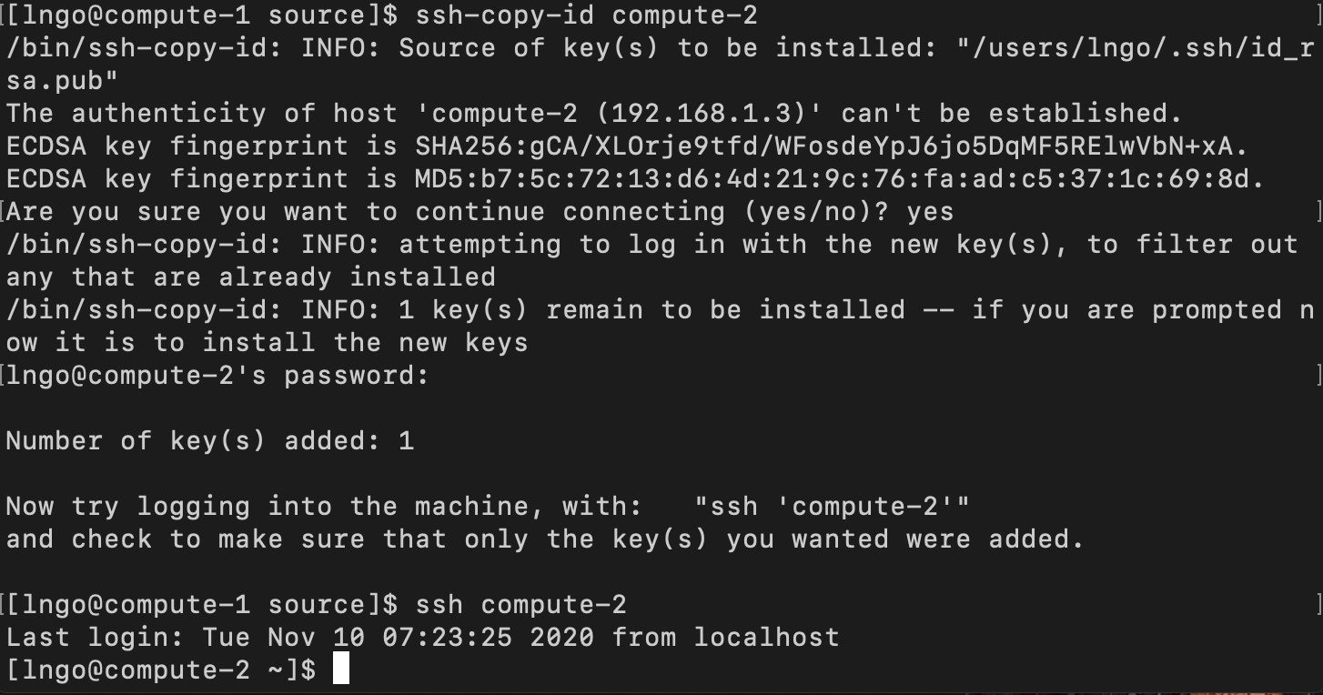
Copy the key from compute-1 to compute-2.

Switch to the terminal that logged onto compute-1

Answer yes if asked about the authenticity of host.

Enter the password for your account on compute-2 (that you setup previously!)

If passwordless SSH was successfully setup, a subsequence SSH from compute-1 to compute-2 will not require any password.

Repeat the process to setup passwordless SSH from compute-2 to compute-1.
$ ssh-copy-id compute-2 
$ ssh compute-2
$ exit
On each node, compute-1 and compute-2, run the followings:
$ echo "export PATH=/opt/openmpi/3.1.2/bin/:$PATH" >> ~/.bashrc 
$ echo "export LD_LIBRARY_PATH=/opt/openmpi/3.1.3/bin/:$LD_LIBRARY_PATH" >> ~/.bashrc
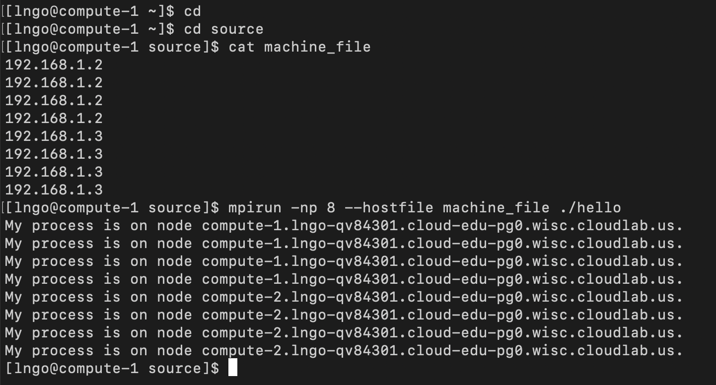
On compute-2, repeat the process to copy source to your home directory and to compile hello.c.

Switch back to the terminal that logged into compute-1.

View the file machine_file inside the source directory and run the MPI job
$ cd
$ cd source
$ cat machine_file
$ mpirun -np 8 --hostfile machine_file ./hello

1. Type of distributed file systems

Networked File System

Allows transparent access to files stored on a remote disk.

Clustered File System

Allows transparent access to files stored on a large remote set of disks, which could be distributed across multiple computers.

Parallel File System

Enables parallel access to files stored on a large remote set of disks, which could be distributed across multiple computers.

2. Networked File System

Sandberg, R., Goldberg, D., Kleiman, S., Walsh, D., & Lyon, B. (1985, June). “Design and implementation of the Sun network filesystem.” In Proceedings of the Summer USENIX conference (pp. 119-130)

Design goals

Machine and operating system independence

Crash recovery

Transparent access

UNIX semantics maintained on client

Reasonable performance (target 80% as fast as local disk)

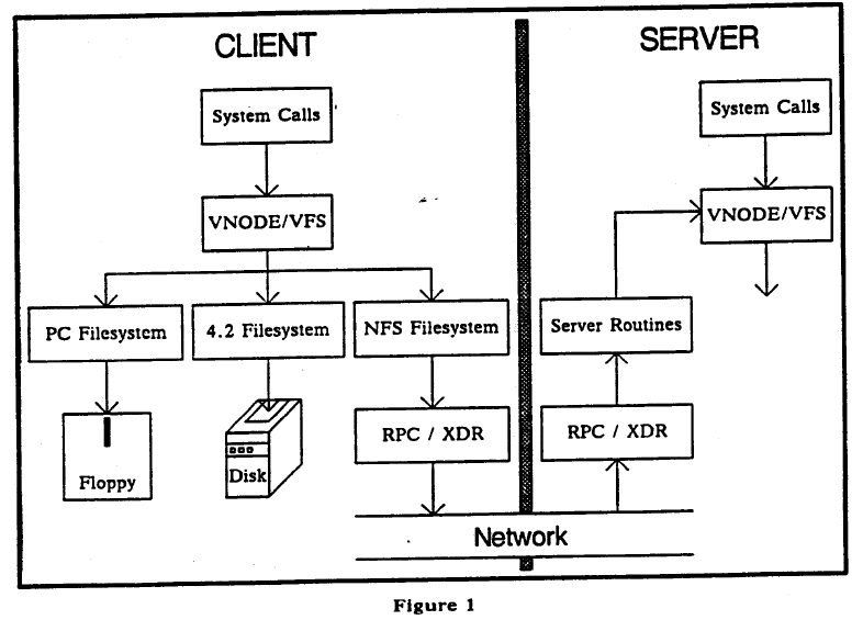
3. Networked File System Design

NFS Protocol

Remote Procedure Call mechanism

Stateless protocol

Transport independence (UDP/IP)

Server side

Must commit modifications before return results

Generation number in inode and filesystem id in superblock

Client side

Additional virtual file system interface in the Linux kernel.

Attach remote file system via mount

4. Clustered File Systems

Additional middleware layers such as the tasks of a file system server can be distributed among a cluster of computers.

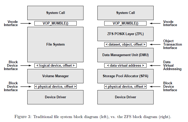
Example: The Zettabyte File System (ZFS) by Sun Microsystem

Bonwick, Jeff, Matt Ahrens, Val Henson, Mark Maybee, and Mark Shellenbaum. “The zettabyte file system.” In Proc. of the 2nd Usenix Conference on File and Storage Technologies, vol. 215. 2003.

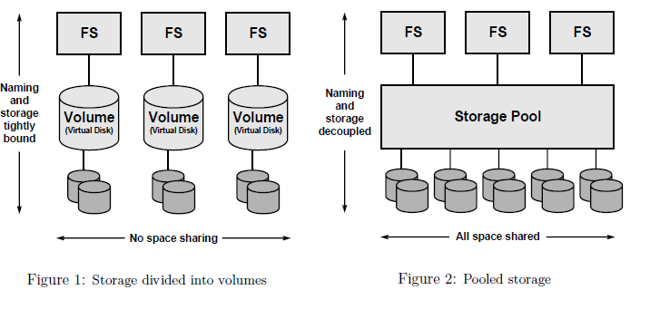
“One of the most striking design principles in modern file systems is the one-to-one association between a file system and a particular storage device (or portion thereof). Volume managers do virtualize the underlying storage to some degree, but in the end, a file system is still assigned to some particular range of blocks of the logical storage device. This is counterintuitive because a file system is intended to virtualize physical storage, and yet there remains a fixed binding between a logical namespace and a specific device (logical or physical, they both look the same to the user).”

5. Clustered File Systems: design principles

Simple administration: simplify and automate administration of storage to a much greater degree.

Pooled storage: decouple file systems from physical storage with allocation being done on the pooled storage side rather than the file system side.

Dynamic file system size

Always consistent-disk data.

Immense capacity (Prediction in 2003: 16 Exabyte datasets to appear in 10.5 years).

Error detection and correction

Integration of volume manager

Excellent performance

6. Parallel File Systems

Ross, Robert, Philip Carns, and David Metheny. “Parallel file systems.” In Data Engineering, pp. 143-168. Springer, Boston, MA, 2009.

“… The storage hardware selected must provide enough raw throughput for the expected workloads. Typical storage hardware architectures also often provide some redundancy to help in creating a fault tolerant system. Storage software, specifically file systems, must organize this storage hardware into a single logical space, provide efficient mechanisms for accessing that space, and hide common hardware failures from compute elements.
Parallel file systems (PFSes) are a particular class of file systems that are well suited to this role. This chapter will describe a variety of PFS architectures, but the key feature that classifies all of them as parallel file systems is their ability to support true parallel I/O. Parallel I/O in this context means that many compute elements can read from or write to the same files concurrently without significant performance degradation and without data corruption. This is the critical element that differentiates PFSes from more traditional network file systems …”

7. Parallel File Systems: fundamental design concepts

Single namespace, including files and directories hierarchy.

Actual data are distributed over storage servers.

Only large files are split up into contiguous data regions.

Metadata regarding namespace and data distribution are stored:

Dedicated metadata servers (PVFS)

Distributed across storage servers (CephFS)

8. Parallel File Systems: access mechanism

Shared-file (N-to-1): A single file is created, and all application tasks write to that file (usually to disjoint regions)

Increased usability: only one file is needed

Can create lock contention and reduce performance

File-per-process (N-to-N): Each application task creates a separate file, and writes only to that file.

Avoids lock contention

Can create massive amount of small files

Does not support application restart on different number of tasks

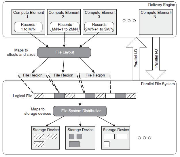
9. Parallel File Systems: data distribution

Original File: Sequence of Bytes

Sequence of bytes are converted into sequence of offsets (each offset can cover multiple bytes)

Offsets are mapped to objects

not necessarily ordered mapping

reversible to allow clients to contact specific PFS server for specific data content

Objects are distributed across PFS servers

Information about where the objects are is stored at the metadata server

10. Parallel File Systems: object placement

Round robin is reasonable default solution

Work consistently on most systems

Default solutions for: GPFS, Lustre, PVFS

Potential scalability issue with massive scaling of file servers and file size

Two dimensional distribution

Limit number of servers per file

11. Design challenges

Performance

How well the file system interfaces with applications

Consistency Semantics

Interoperability:

POSIX/UNIX

MPI/IO

Fault Tolerance:

Amplifies due to PFS’ multiple storage devices and I/O Path

Management Tools

12. Hands-on: Setup NFS

Log into CloudLab
Log into the head node on your cluster
Run the following bash commands from your home directory:

$ sudo yum install -y nfs-utils
$ sudo mkdir -p /scratch
$ sudo chown nobody:nobody /scratch
$ sudo chmod 777 /scratch
$ sudo systemctl enable rpcbind
$ sudo systemctl enable nfs-server
$ sudo systemctl enable nfs-lock
$ sudo systemctl enable nfs-idmap
$ sudo systemctl start rpcbind
$ sudo systemctl start nfs-server
$ sudo systemctl start nfs-lock
$ sudo systemctl start nfs-idmap
$ echo "/scratch 192.168.1.2(rw,sync,no_root_squash,no_subtree_check)" | sudo tee -a /etc/exports
$ echo "/scratch 192.168.1.3(rw,sync,no_root_squash,no_subtree_check)" | sudo tee -a /etc/exports
$ sudo systemctl restart nfs-server

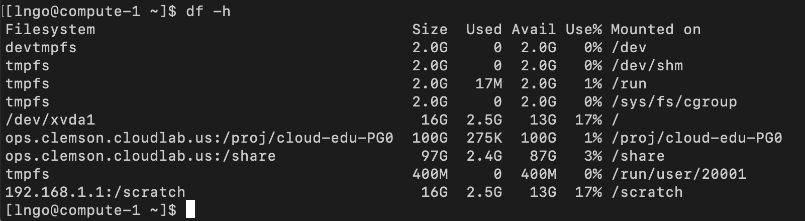
Log into compute-1 and compute-2 nodes on your cluster
Run the following bash commands from your home directory on both nodes:

$ echo "export PATH=/opt/openmpi/3.1.2/bin/:$PATH" >> ~/.bashrc 
$ echo "export LD_LIBRARY_PATH=/opt/openmpi/3.1.2/bin/:$LD_LIBRARY_PATH" >> ~/.bashrc
$ sudo yum install -y nfs-utils
$ sudo mkdir -p /scratch
$ sudo mount -t nfs 192.168.1.1:/scratch /scratch
$ df -h

NFS mount

On compute-1, run the followings

$ cd 
$ ssh-keygen -t rsa -f .ssh/id_rsa -N ''
$ cat .ssh/id_rsa.pub >> .ssh/authorized_keys
$ cp -R .ssh /scratch

On compute-2, run the following

$ cp -R /scratch/.ssh .

{: .language-bash}>

Test passwordless SSH by attempting to SSH to compute-1 from compute-2 and vice versa.
Log on to compute-1 and run the followings:

$ cd /scratch
$ cp -R /local/repository/source .
$ cd source
$ mpicc -o hello hello.c 
$ mpirun -np 8 --hostfile machine_file ./hello

Key Points

Schedulers for cluster of computers

Overview

Teaching: 0 min
Exercises: 0 min

Questions

What does it mean to schedule jobs on a supercomputer?

Objectives

1. Introduction

The term scheduling impacts several levels of the system, from application/task scheduling which deals with scheduling of threads to meta-scheduling where jobs are scheduled across multiple supercomputers.

Here, we focus on job-scheduling, scheduling of jobs on a supercomputer, the enabling software infrastructure and underlying algorithms.

This is an optimization problem in packing with space (processor) and time constraints

Dynamic environment

Tradeoffs in turnaround, utilization, and fairness

2. Introduction: Job scheduling

Simplest way to schedule in a parallel system is using a queue

Each job is submitted to a queue and each job upon appropriate resource match executes to completion while other jobs wait.

Since each application utilizes only a subset of systems processors, the processors not in the subset could potentially remain idle during execution. Reduction of unused processors and maximization of system utilization is the focus of much of scheduling research.

Space Sharing: A natural extension of the queue where the system allows for another job in the queue to execute on the idle processors if enough are available.

Time Sharing: Another model where a processor’s time is shared among threads of different parallel programs. In such approaches each processor executes a thread for some time, pauses it and then begins executing a new thread. Eg. Gang Scheduling

Since context switching in Time Sharing involves overhead,complex job resource requirements and memory management, most supercomputing installations prefer space sharing scheduling systems.

3. CPU scheduling

Scheduling of CPUs is fundamental to Operating System design

Process execution consists of a cycle of CPU execution and I/O wait. The process execution begins with a CPU burst followed by an I/O burst etc.

OS selects one of the processes from the short term scheduler / CPU scheduler.

The scheduler selects from among the process in memory that are ready to execute and allocates the CPU to one of them.

Scheduling happens under one of 4 conditions:

When process switches from running state to the waiting state (Non Preemptive)

When a process switches from the running state to the ready state (Preemptive)

When a process switches from the waiting state to the ready state (Preemptive)

When a process terminates (Non Preemptive)

4. CPU scheduling

Scheduling Criteria:

MAX CPU Utilization needs to keep the CPU as busy as possible.

MAX Throughput Number of processes completed per time unit

MIN Turnaround Time the interval from the time of submission of a process to the time of completion

MIN Waiting Time Sum of the periods spent by the process waiting in the ready queue

MIN Response Time The measure of time from the submission of a request until the first response is produced

5. Workload management systems

Supercomputing Centers often support several hundreds of users running thousands of jobs across a shared supercomputing resources consisting of large number of compute nodes and storage centers.

It can be extremely difficult for an administrator of such a resource to manually manage users, resource allocations and ensure optimal utilization of the large supercomputing resources.

Workload management systems (WMS) help address this problem by providing users with simple resource access and for the administrator of the supercomputing resource, a set of powerful tools and utilities for resource management, monitoring, scheduling, accounting, and policy enforcement.

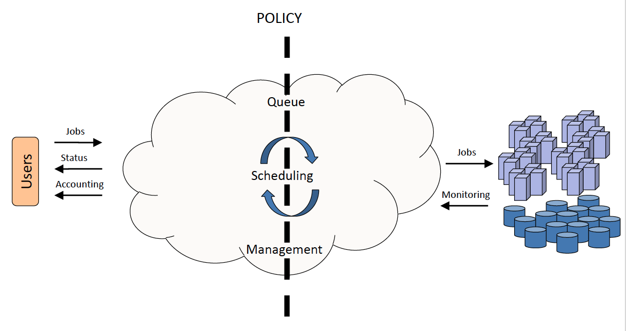
6. Workload management systems: main activities

Queuing

Scheduling

Monitoring

Resource Management

Accounting

7. Workload management systems: a layer between users and computing resources

Users submit jobs, specifying the work to be performed, to a queue

Jobs wait in queue until they are scheduled to start on the cluster.

Scheduling is governed by stipulated policies and algorithms that implement the policy. (Policies usually ensure fair sharing of resources and attempt to optimize overall system utilization.)

Resource management mechanisms handle launching of jobs and subsequent cleanup.

The workload management system is simultaneously monitoring the status of various system resources and accounting resource utilization.

8. Workload management systems: queueing

The most visible part of the WMS process where the system collects the jobs to be executed.

Submission of jobs is usually performed in a container called a batch job (usually specified in the form of a file).

The batch job consists of two primary parts :

A set of resource directives (number of CPUs, amount of memory etc.)

A description of the task(s) to be executed (executable, arguments etc.)

Upon submission the batch job is held in a queue until a matching resource is found. Queue wait time for submitted jobs could vary depending on the demand for the resource among users.

Production or real world supercomputing resources often have multiple queues, each of which can be preconfigured to run certain kinds of jobs. ExampleTezpurcluster has a debug queue and workq

9. Workload management systems: scheduling

Scheduling selects the best job to run based on the current resource availability and scheduling policy.

Scheduling can be generally broken into two primary activities :

Policy enforcement : To enforce resource utilization based on policies set by supercomputing sites (controls job priority and schedulability).

Resource Optimization : Packs jobs efficiently, and exploit underused resources to boost overall resource utilization.

Balancing policy enforcement with resource optimization in order to pick the best job to run is the difficult part of scheduling

Common scheduling algorithms include First In First Out, Backfill, Fairshare.

10. Workload management systems: monitoring

Resource monitoring by WMS, provides administrators, users and scheduling systems with status information of jobs and resources. Monitoring is often performed for 3 critical states:

For idle nodes , to verify their working order and readiness to run another job.

For busy nodes , to monitor memory, CPU, network, I/O and utilization of system resources to ensure proper distribution of workload and effective utilization of nodes.

For completed jobs , to ensure that no processes remain from the completed job and that the node is still in working order before a new job is started on it.

11. Workload management systems: resource management

Resource Management area is responsible for starting, stopping, and cleaning up after jobs.

A batch system resource management is setup in such a way so as to run the jobs using the identity of a user in such a way that the user need not be present at that time.

Jobs are started only on the nodes that are functioning properly.

Resource management also includes removing or adding of resources to the available pool of systems

Clusters are dynamic resources, systems go down, or additional resources are added.

Registration of new nodes and the marking of nodes as unavailable are additional aspects of resource management

12. Workload management systems: accounting and reporting

Workload accounting can be defined as the process of collecting resource usage data for the batch jobs that run on the resource. (example % CPU utilization, memory utilization etc.)

Data obtained from accounting is often used to :

Produce weekly/monthly per user usage reports

Tuning of scheduling policy

Calculating future resource allocations

Anticipating future computer component requirements

Determining areas for improvement within the system.

13. Scheduling algorithm: FCFS/FIFO

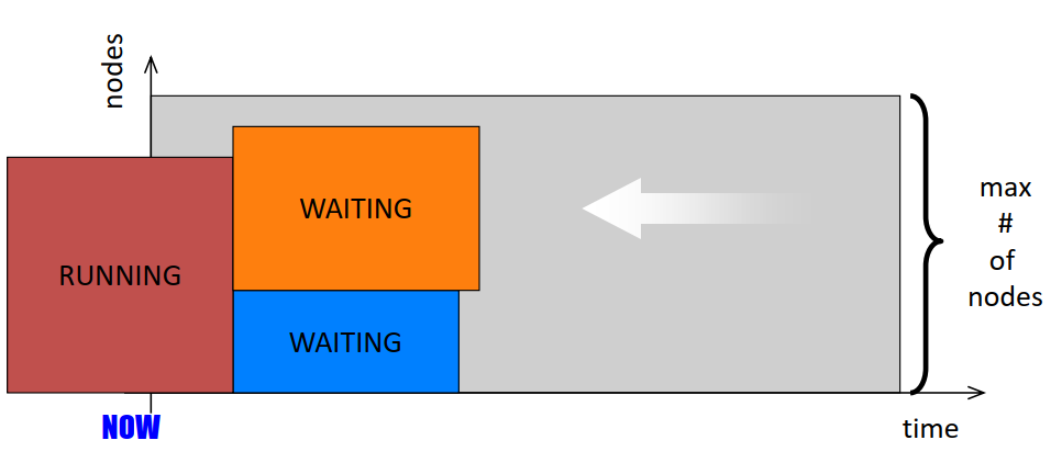
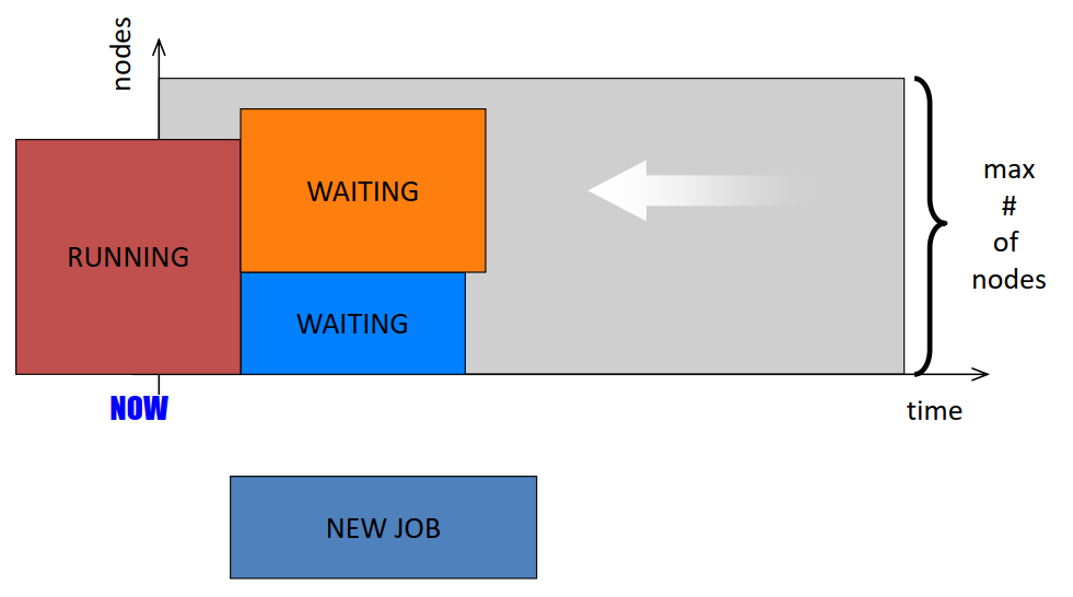
Definitions

Shadow time: time at which the first job in the queue starts execution

Extra nodes: number of nodes idle when the first job in the queue starts execution

Simplest scheduling option: FCFS

First Come First Serve

Problem:

Fragmentation:

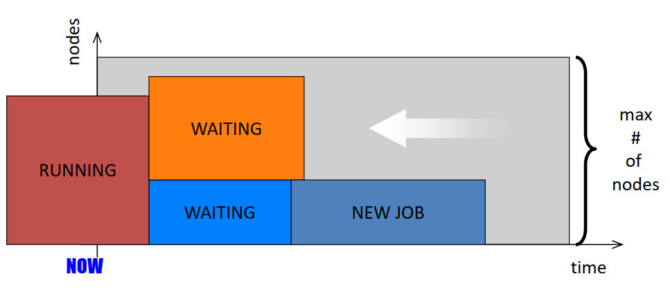
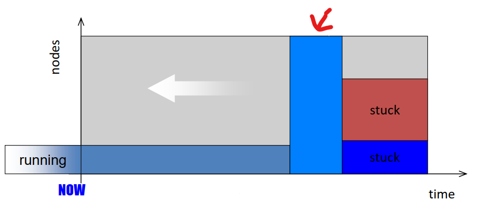
14. Scheduling algorithm: FCFS with Backfilling

Which job(s) should be picked for promotion through the queue?

Many heuristics are possible

Two have been studied in detail

EASY

Conservative Back Filling (CBF)

In practice EASY (or variants of it) is used, while CBF is not

Extensible Argonne Scheduling System

Maintain only one “reservation”, for the first job in the queue

Go through the queue in order starting with the 2nd job

Backfill a job if

it will terminate by the shadow time, or

it needs less than the extra nodes

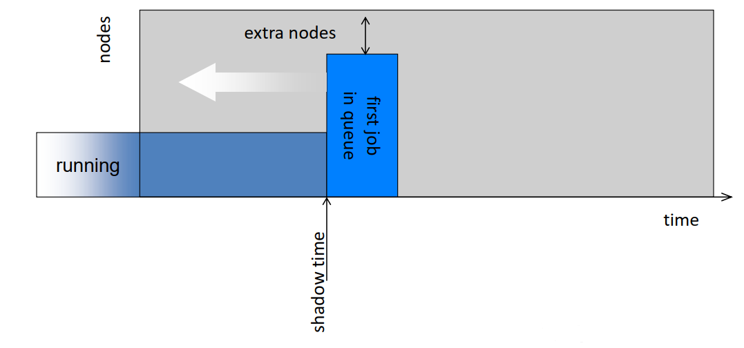
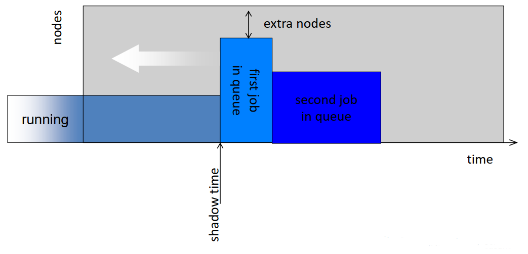
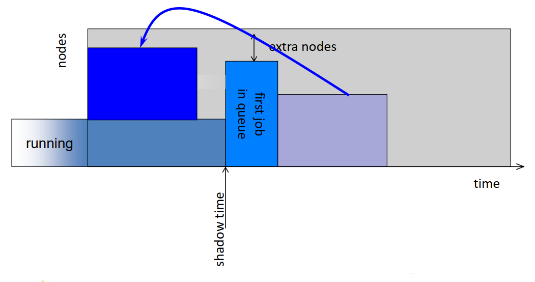
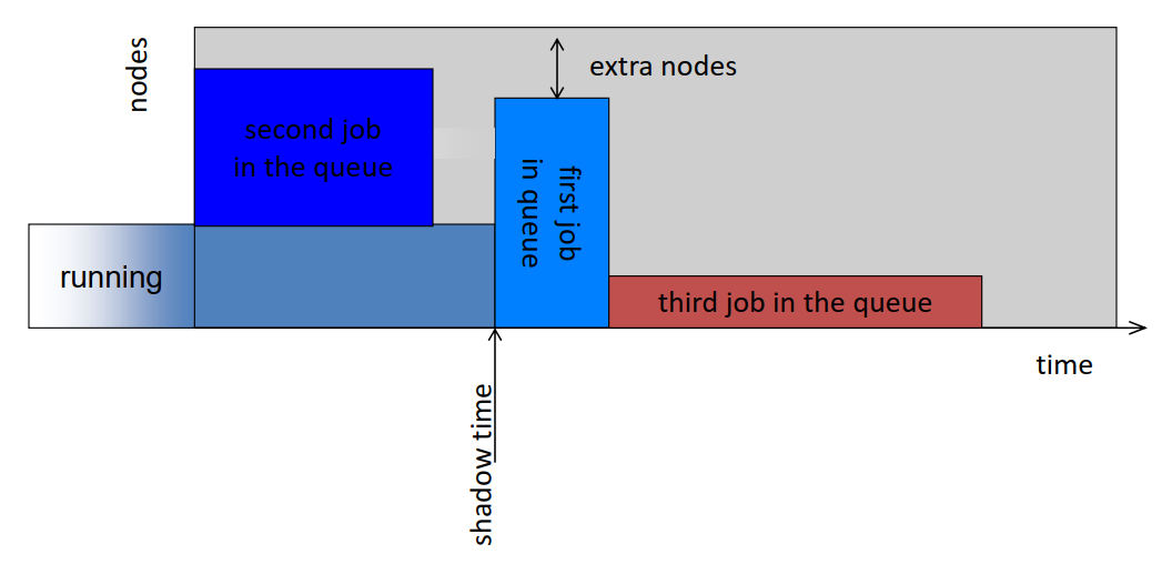
Problem:

The first job in the queue will never be delayed by backfilled jobs

BUT, other jobs may be delayed infinitely!

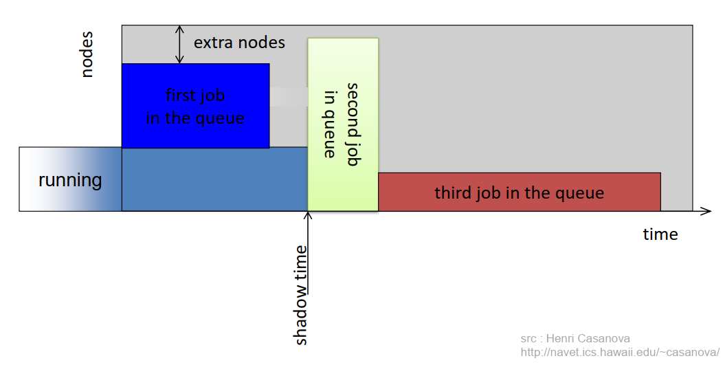
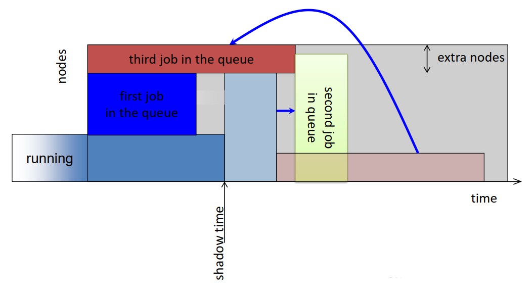
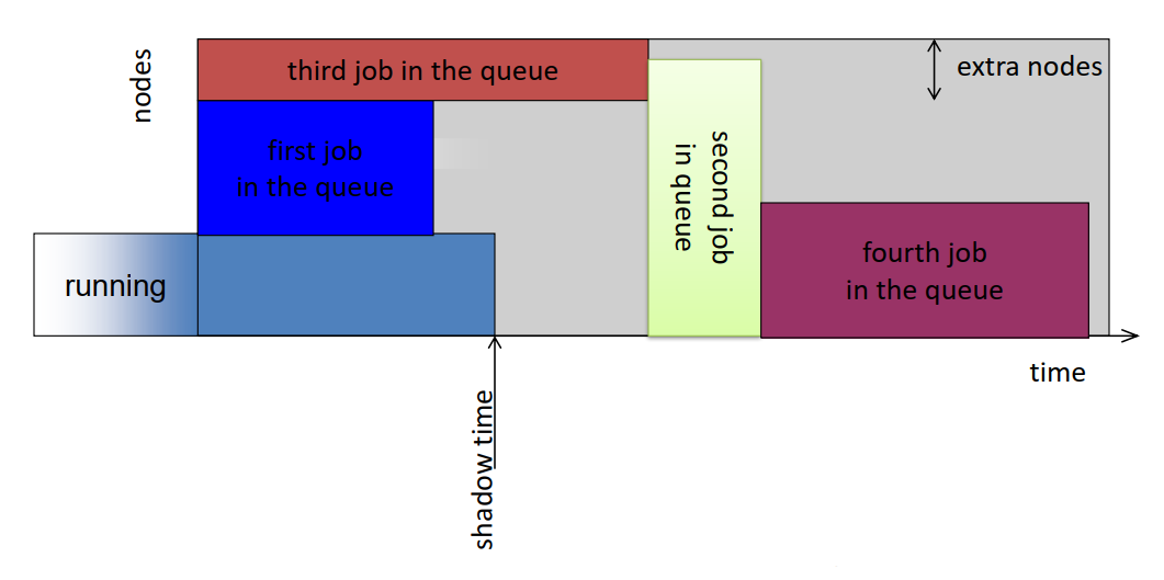
Unbounded Delay

The first job in the queue will never be delayed by backfilled jobs

BUT, other jobs may be delayed infinitely!

No starvation

Delay of first job is bounded by runtime of current jobs

When the first job runs, the second job becomes the first job in the queue

Once it is the first job, it cannot be delayed further

EASY favors small long jobs

EASY harms large short jobs

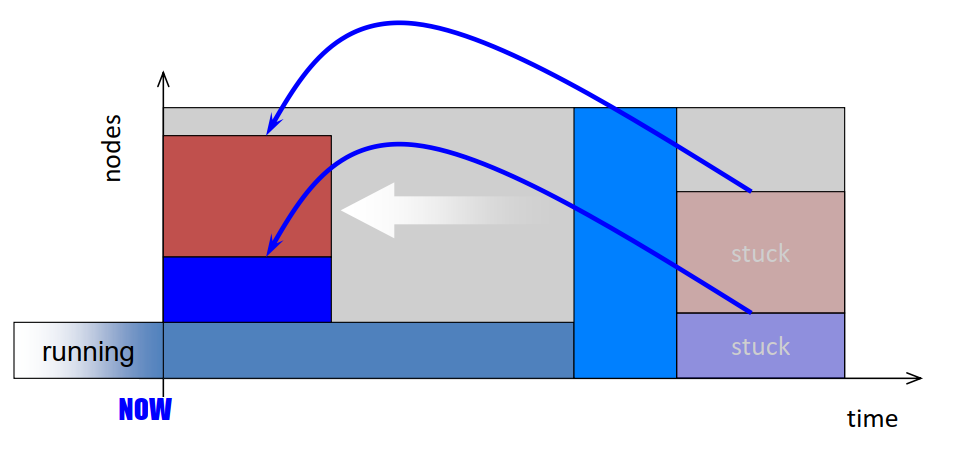
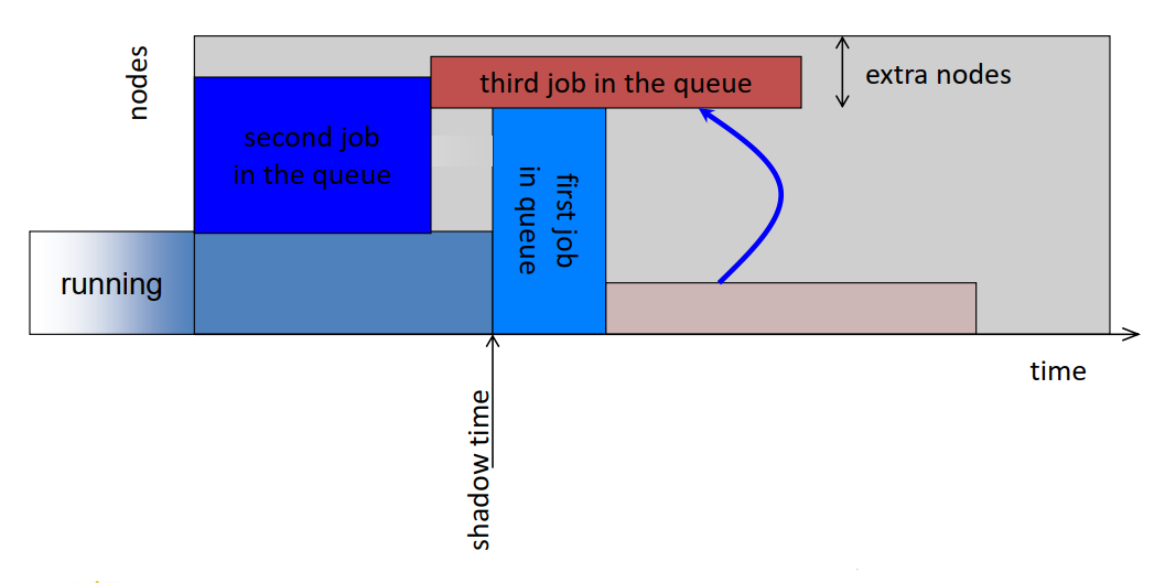
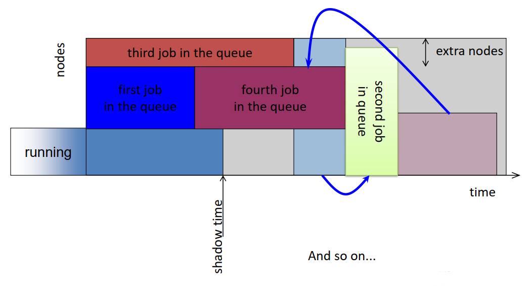
15. Conservative Backfilling

EVERY job has a “reservation”

A job may be backfilled only if it does not delay any other job ahead of it in the queue.

Fixes the unbounded delay problem that EASY has

More complicated to implement: The algorithm must find holes in the schedule

16. How good is the schedule?

All of this is great, but how do we know what a good schedule is?

FCFS, EASY, CFB, Random?

What we need are metrics to quantify how good a schedule is

It has to be an aggregate metric over all jobs

Metric #1: Turn-around time

Also called flow

Wait time + Run time

But:

Job #1 needs 1h of compute time and waits 1s

Job #2 needs 1s of compute time and waits 1h

Clearly Job #1 is really happy, and Job #2 is not happy at all

Metric #2: wait time

But

Job #1 asks for 1 node and waits 1 h

Job #2 asks for 512 nodes and waits 1h

Again, Job #1 is unhappy while Job #2 is probably sort of happy

17. SLURM Scheduler

Work funded by Department of Energy at Lawrence Livermore National Laboratory.

SLURM: Simple Linux Utility for Resource Management.

SLURM characteristics:

Simple

Open source

Portable (written in C, requires no kernel modification)

Fault-tolerant

Secure

System administrator friendly

Scalable (16K nodes, 128K processors)

18. SLURM Scheduler: entities

Nodes: Individual computers

Partitions: Job queues

Jobs: Resource allocations

Job steps: Set of (typically parallel) tasks

19. SLURM Scheduler: job states

Jobs:

Resource allocation: specific processors and memory or entire nodes allocated to a user for some time period.

Can be interactive (executed in real-time) or batch (script queued for later execution).

Many constraints available for user request

Identified by ID number

Job steps:

A set of tasks launched at the same time and sharing a common communication mechanism (e.g. switch windows configured for the tasks).

Allocated resources within the job’s allocation

Multiple job steps can executed concurrently or sequentially on unique or overlapping resources

Identified by ID number: jobid.stepid

20. SLURM Scheduler: control daemon and compute node daemon

Control daemon: slurmctld

Orchestrates SLURM activities across the cluster

Primary components

Node Manager: Monitors node state

Partition Manager: Groups nodes into partitions with various configuration parameters and allocates nodes to jobs

Job Manager: Accepts user job requests and places pending jobs into priority-ordered queue. Uses the partition manager to allocate resources to the jobs and then launch them.

Compute node daemon: slurmd

Monitors state of a single node

Manages user jobs and job steps within that node

Very light-weight

Supports hierarchical communications with configurable fanout (new in version 1.1)

Key Points

Data intensive computing

Overview

Teaching: 0 min
Exercises: 0 min

Questions

Objectives

Key Points

High throughput computing

Overview

Teaching: 0 min
Exercises: 0 min

Questions

Objectives

Key Points

Introduction to IOT

Overview

Teaching: 0 min
Exercises: 0 min

Questions

Objectives

Key Points

Distributed and Cluster Computing

The demand for computational speed

Overview

How do we measure speed in computation?

Modern measurement of speed

The bragging list (The TOP500 Project)

Why do we need this much speed?

Faster computer gives more details

Hurricane Sandy (2012)

Various forecasts of Sandy

One of the contributing factors

The US has catched up

Covid and HPC

Manufacturing and HPC

Oil and Gas Expoloration improvement with HPC

Fraud Detection at PayPal

Key Points

Introduction to paralel and distributed computing

Overview

Envision the payroll problem

Components of a computation problem

Parallelizing payroll

Computational tasks should be able to …

Execution framework should be able to …

Computing resources might be …

The progress

Single site, single computer, single core

Single site, single computer, multiple cores

Single site, multiple computers, multiple cores

Multiple sites, multiple computers, multiple cores, federated domains

Multiple site, multiple computers, multiple cores, virtula unified domain

Distributed computing systems

emphasis …

Can we just throw more computers at the problem?

Parallel speedup

Example 1

Solution

Theoretical max

Amdahl’s Law

Parallel efficiency

Example 2

Solution

Example 3

Serial portion

Speedup on 20 processors

Efficiency

Best speedup

Limiting factors of parallel speedup

If there is no limiting factor …

Superlinear speedup

Computer architecture: Flynn’s Taxonomy

Types of distributed computing systems

Streaming SIMD

Shared memory

Heterogeneous computing

GPU - graphics processing unit

FPGA - field programmable array

Co-processors

Message passing distributed computing

Benchmarking

Ranking

Key Points

Introduction to OpenMP

Overview

Target hardware

Target software

Basic requirements to write, compile, and run an OpenMP program

OMP directives

Hands-on 1: Setup directory

Hands-on 2: Create hello_omp.c

What’s important?

Example: trapezoidal

Hands-on 3: Trapezoid implementation

Hands-on 4: A bit more detailed

Challenge 1:

Solution

Challenge 2:

Solution

Challenge 3:

Solution