Introduction to paralel and distributed computing

Overview

Teaching: 0 min
Exercises: 0 min

Questions

• What is parallel computing?

Objectives

• Understand basic architectures and computing models for parallel computing.

• Understand and be able to carry out rudimentary speedup and efficiency study.

Envision the payroll problem

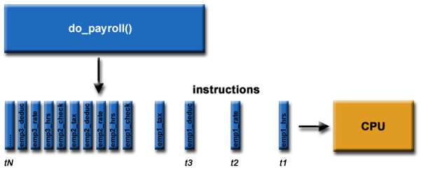
Components of a computation problem

• Computational task
• Execution framework.
• Computing resources.

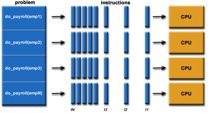
Parallelizing payroll

Computational tasks should be able to …

• Be borken apart into discrete pieces of work that can be solved simultaneously.
• Be solved in less time with multiple computing resources than with a single computing resource.

Execution framework should be able to …

• Execute multiple program instructions concurrently at any moment in time

Computing resources might be …

• A single computer with multiple processors.
• An arbitrary number of computers connected by a network.
• A special computational component inside a single computer, separate from the main processors (GPU), or
• Any combintations of the above.

The progress

How do parallel and distributed computing resources evolve?

Single site, single computer, single core

Single site, single computer, multiple cores

Single site, multiple computers, multiple cores

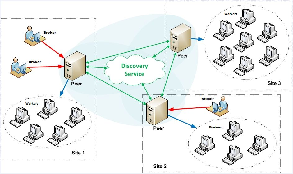
Multiple sites, multiple computers, multiple cores, federated domains

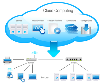
Multiple site, multiple computers, multiple cores, virtula unified domain

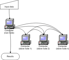
Distributed computing systems

“A collection of individual computing devices that can communicate with each other.” (Attiya and Welch, 2004).

emphasis …

“A collection of individual computing devices that can communicate with each other.” (Attiya and Welch, 2004).

Can we just throw more computers at the problem?

• Parallel speedup: how much faster the program becomes once some computing resources are added.
• Parallel efficiency: Ratio of performance improvement per individual unit of computing resource.

Parallel speedup

• Given p processors,
• Speedup, S(p), is the ratio of the time it takes to run the program using a single processor over the time it takes to run the program using p processors.
• The time it takes to run the program using a single processor, $t_{s}$: sequential run time
• The time it takes to the the program using multiple processor, $t_{p}$: parallel run time $\\\\S(p) = \frac{sequential\ run\ time}{parallel\ run\ time} = \frac{t_s}{t_p}\\$

Example 1

A program takes 30 seconds to run on a single-core machine and 20 seconds to run on a dual-core machine. What is the speedup of this program?

Solution

$t_s=30$
$t_p=20$
$S=\frac{t_s}{t_p}=\frac{30}{20}=1.5$

Theoretical max

• Let f be the fraction of the program that is not parallelizable.
• Assume no overhead.
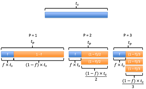
• Running the program using one processor will take time $t_s$.
• The parallel run time, $t_p$, can be calculated as the time it take to run the fraction that is non-parallelizable ($f\times t_s$) plus the remainning parallelizable fraction ($1-f$).
• If $p=1$, this simplifies to $t_p=f\times t_s + (1-f)\times t_s$.
• Assume no overhead, this means that we reduce the speed by half as we double the number of processor.
• And so on …

Amdahl’s Law

• This brings us to Amdahl’s Law, which quantifies speedup in term of number of processors and fraction of non-parallelizable code:
  $S(p)=\frac{t_s}{t_p}=\frac{t_s}{f\times t_s + (1-f)\times t_s}=\frac{1}{f + \frac{1-f}{p}}=\frac{p}{f \times (p-1) + 1}$

Parallel efficiency

• The efficiency E is then defined as the ratio of speedup S(p) over the number of processors p.
  $E=\frac{\frac{p}{f \times (p-1) + 1}}{p}=\frac{1}{f \times (p-1) + 1}$
• E is often measured as percentage.
• For example, E = 0.8 means the parallel efficiency is 80%.

Example 2

Suppose that 4% of my application is serial. What is my predicted speedup according to Amdahl’s Law on 5 processors?

Solution

$f=0.04$
$p=5$
$S=\frac{p}{(p-1)f + 1}=\frac{5}{4 \times 0.4 +1}=1.9231$

Example 3

Suppose that I get a speedup of 8 when I run my application on 10 processors. According to Amdahl’s Law:

• What portion of my code is serial?
• What is the speedup on 20 processors?
• What is the efficiency on 5 processors? 20 processors?
• What is the best speedup that I could achieve?

Serial portion

$S=8$
$p=10$
$S=\frac{p}{(p-1)f + 1}$
$8=\frac{10}{9f+1}$
$9f + 1 = \frac{10}{8}$
$f=\frac{1}{36}$

Speedup on 20 processors

$f=\frac{1}{36}$
$p=20$
$S_{20}=\frac{p}{(p-1)f + 1}=\frac{20}{\frac{19}{36}+1} \approx 13.0909$

Efficiency

$E=\frac{1}{(p-1)f + 1}$
$E_5=\frac{1}{\frac{4}{36}+1} = 90\%$
$E_{20}=\frac{1}{\frac{19}{36} + 1} \approx 65.45\%$

Best speedup

$f=\frac{1}{36}$
$S_{\infty}=\lim_{p \to +\infty} \frac{p}{(p-1)f + 1} = \lim_{p \to +\infty} \frac{1}{\frac{p}{p-1}f + \frac{1}{p}}=\frac{1}{f}$
$S_{\infty}= 36$

• In other word, the highest number of processors one should add to this problem is 36.

Limiting factors of parallel speedup

• Non-parallelizable code.
• Communication overhead.

If there is no limiting factor …

• 0% non-paralellizable code.
• No communication overhead.
  $S_{\infty}=\lim_{f \to 0} \frac{p}{(p-1)f + 1} = p$
  $S \leq p$

Superlinear speedup

• The unicorn of parallel and distributed computing.
• Poor sequential reference implementation.
• Memory caching.
• I/O blocking.

Computer architecture: Flynn’s Taxonomy

Types of distributed computing systems

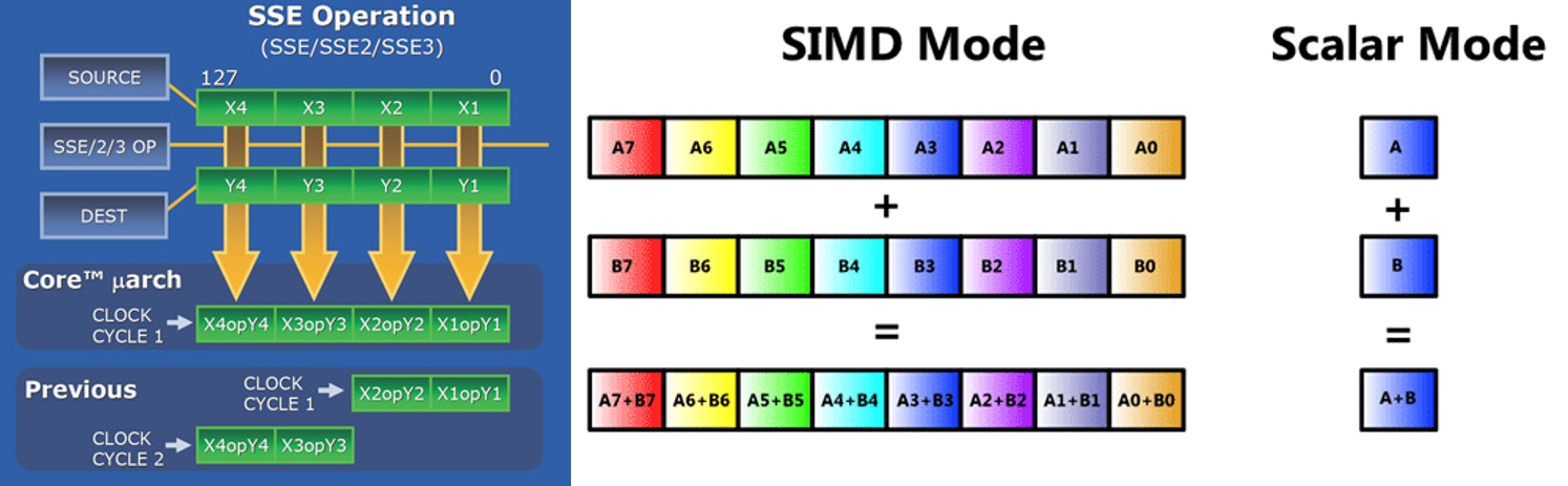
• Streaming SIMD extensions for x86 architectures.
• Shared memory.
• Distributed shared memory.
• Heterogeneous computing (accelerators).
• Message passing.

Streaming SIMD

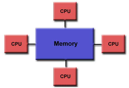
Shared memory

• One processor, multiple threads.
• All threads have read/write access to the same memory.
• Programming models:
  • Threads (pthread) - programmer manages all parallelism.
  • OpenMP: compiler extensions handle.
  • Vendor libraries: (Intel MKL - math kernel libraries)

Heterogeneous computing

• GPU
• FPGA
• Co-processors

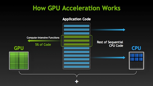
GPU - graphics processing unit

• Processor unit on graphic cards designed to support graphic rendering (numerical manipulation).
• Significant advantage for certain classes of scientific problems.
• Programming models:
  • CUDA: Library developed by NVIDIA for their GPUs.
  • OpenACC: Standard developed by NVIDIA, Cray, and Portal Compiler (PGI).
  • OpenAMP: Extension to Visual C++ to direct computation to GPU.
  • OpenCL: Public standard by the group the developed OpenGL.

FPGA - field programmable array

• Dynamically reconfigurable circuit board.
• Expensive, difficult to program.
• Power efficient, low heat.

Co-processors

• Enables offloading of computationally intensive tasks from main CPU.
• Similar to GPU, but can support a wider range of computational tasks.
• Intel
  • Xeon Phi processor line.
  • PCIe-based add-on cards, but could also be used as a stand alone CPU.
  • Unlike GPU, Intel Xeon supports all programs targeted to standard x86 CPU (very minor modification if any)

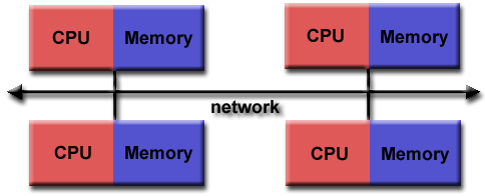
Message passing distributed computing

• Processes handle their own memory.
• Data is passed between processes via messages.
  • Scales well.
  • Cluster can be built from commodity parts.
  • Cluster can easily be expanded.
  • Cluster can be heterogeneous.
• Programming models:
  • MPI: standardized message passing library.
  • MPI + OpenMP: hybrid model.
  • MapReduce programming model for big data processing.
    

Benchmarking

• LINPACK (Linear Algebra Package): Dense Matrix Solver
• HPCC: High-Performance Computing Challenge.
  • HPL (LINPACK to solve linear system of equations)
  • DGEMM (Double precision general matrix multiply)
  • STREAM (Memory bandwidth)
  • PTRANS (Parallel matrix transpose to measure processors communication)
  • RandomAccess (random memory updates)
  • FFT (double precision complex discrete fourier transform)
  • Communication bandwidth and latency
• SHOC: Scalable heterogeneous computing
  • Non-traditional system (GPU)
• TestDFSIO
  • I/O performance of MapReduce/Hadoop Distributed File System.

Ranking

• TOP500: Rank the supercomputers based on their LINPACK score.
• GREEN500: Rank the supercomputers with emphasis on energy usage (LINPACK/power consumption).
• GRAPH500: Rank systems based on benchmarks designed for data-intensive computing.

Key Points

• There various parallel computing architecture/model

• Users need to find the one that give the best speedup/efficiency measures.

• Speed/efficiency depends on how well programs are parallelized.