Introduction

Overview

Teaching: 0 min
Exercises: 0 min

Questions

• What is the big picture?

Objectives

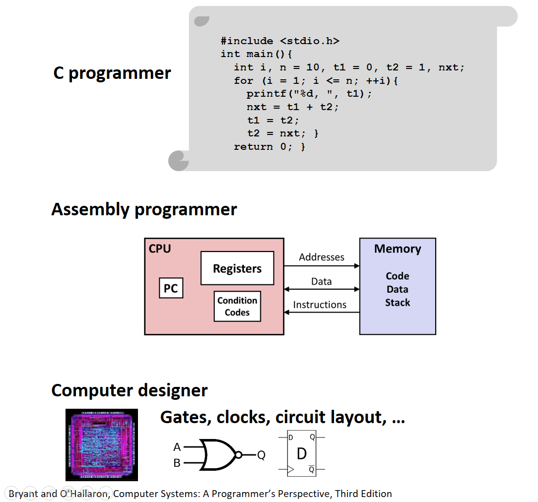
• Know how hardware and software interact through (programming) interfaces.

• Know different types of systems programs.

1. Overview

• Systems knowledge is power!
  • How hardware (processors, memories, disk drives, network infrastructure) plus software (operating systems, compilers, libraries, network protocols) combine to support the execution of application programs.
  • How general-purpose software developers can best use these resources.
  • A new specialization: systems programming.

2. Understand how things work

• Why do I need to know this stuff?
  • Abstraction is good, but don’t forget reality
• Most CS courses emphasize abstraction
  • Abstract data types
  • Asymptotic analysis
• These abstractions have limits
  • Especially in the presence of bugs
  • Need to understand details of underlying implementations
  • Sometimes the abstract interfaces don’t provide the level of control or performance you need

3. Hands-on: Getting started

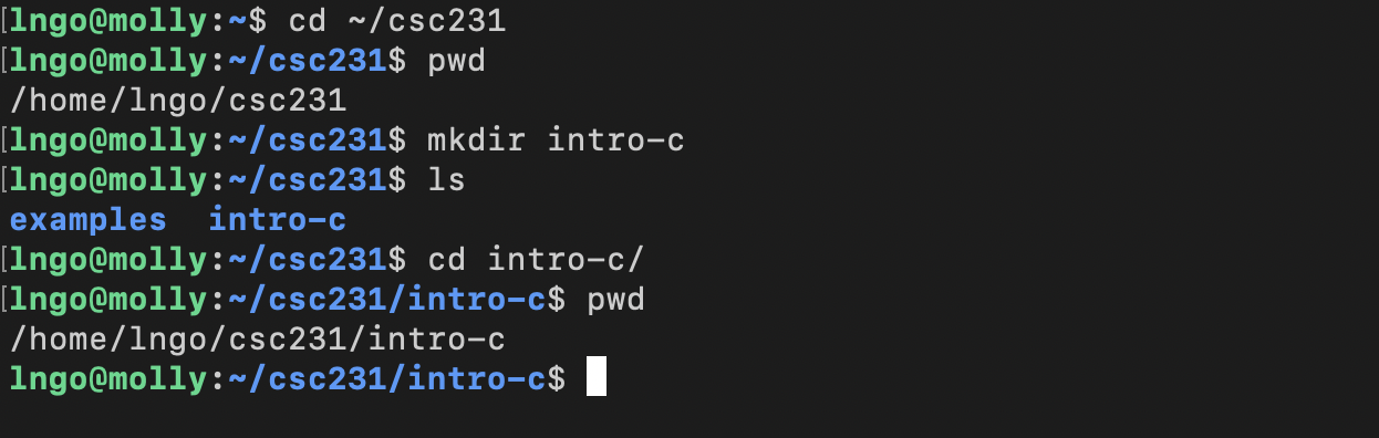
Log into molly and run the following commands:

• Create a directory called csc231 in your home directory using the mkdir command.
• Change into that directory using the cd command.
• The $ sign is not part of the command, but it indicates that the command is to be executed from a command line terminal prompt.

  $ mkdir csc231
  $ cd csc231
  

• Check that you are inside csc231 using the pwd command.
• Clone the Git repository for the class’ examples.

$ pwd
$ git clone https://github.com/CSC231-WCU/examples.git

• The git clone command will download the repository into a directory called examples inside your current directory, which is csc231.
• Run the command ls -l to confirm that examples exists.
• Change into examples using cd.
• Run ls -l to see how many subdirectories there are inside examples.

$ ls -l
$ cd examples
$ ls -l

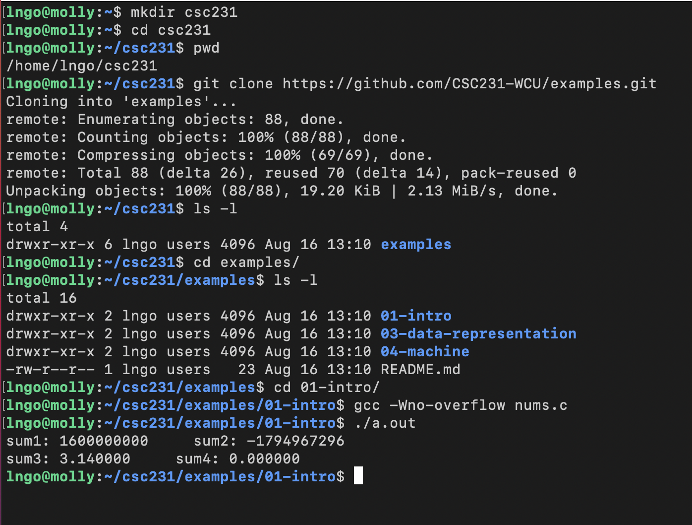
• Change into the directory 01-intro.
• Compile and run the example code nums.c.

$ cd 01-intro
$ gcc -Wno-overflow nums.c
$ ./a.out

4. Computer arithmetic

• Does not generate random values
  • Arithmetic operations have important mathematical properties.
• Cannot assume all usual mathematical properties.
  • Due to finiteness of representations.
  • Integer operations satisfy ring properties: commutativity, associativity, distributivity.
  • Floating point operations satisfy ordering properties: monotonicity, values of signs.
• Observation
  • Need to understand which abstractions apply in which contexts.
  • Important issues for compiler writers and application programmers.

5. Assembly

• You are more likely than not to never write programs in assembly.
  • Compilers take care of this for you.
• Understand assembly is key to machine-level execution model.
  • Behavior of programs in presence of bugs
    • High-level language models break down
  • Tuning program performance
    • Understand optimizations done / not done by the compiler
    • Understanding sources of program inefficiency
  • Implementing system software
    • Compiler has machine code as target
    • Operating systems must manage process state
  • Creating / fighting malware
    • x86 assembly is the language of choice!

6. Memory Matters

• Random Access Memory is an unphysical abstraction.
• Memory is not unbounded.
  • It must be allocated and managed.
  • Many applications are memory dominated.
• Memory referencing bugs are especially pernicious
  • Pernicious: having a harmful effect, especially in a gradual or subtle way.
  • Effects are distant in both time and space.
• Memory performance is not uniform.
  • Cache and virtual memory effects can greatly affect program performance.
  • Adapting program to characteristics of memory system can lead to major speed improvements

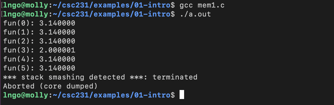
7. Hands-on: Memory referencing bug

• We are still inside examples\intro-01 directory from Hands-on 1.

$ gcc mem1.c
$ ./a.out

8. Memory referencing errors

• C and C++ do not provide any memory protection
  • Out of bounds array references
  • Invalid pointer values
  • Abuses of malloc/free
• Can lead to nasty bugs
  • Whether or not bug has any effect depends on system and compiler
  • Action at a distance
    • Corrupted object logically unrelated to one being accessed
    • Effect of bug may be first observed long after it is generated
• How can I deal with this?
  • Program in Java, Ruby, Python, ML, …
  • Understand what possible interactions may occur
  • Use or develop tools to detect referencing errors (e.g. Valgrind)

9. Beyond asymptotic complexity

• Constant factors matter!
• Exact op count does not predict performance.
  • Possible 10:1 performance range depending on how code written (given same op count).
  • Optimizations must happen at multiple level: algorithm, data representations, procedures, and loop.
• Must understand system to optimize performance
  • How programs compiled and executed.
  • How to measure program performance and identify bottlenecks.
  • How to improve performance without destroying code modularity and generality.

10. Hands-on: Memory system performance

• We are still inside examples\intro-01 directory from Hands-on 1.

$ gcc mem2.c
$ ./a.out

11. Does computer just execute arithmetic and control flow operations?

• They need to get data in and out
  • I/O system critical to program reliability and performance
• They communicate with each other over networks
  • Many system-level issues arise in presence of network
  • Concurrent operations by autonomous processes
  • Coping with unreliable media
  • Cross platform compatibility
  • Complex performance issues

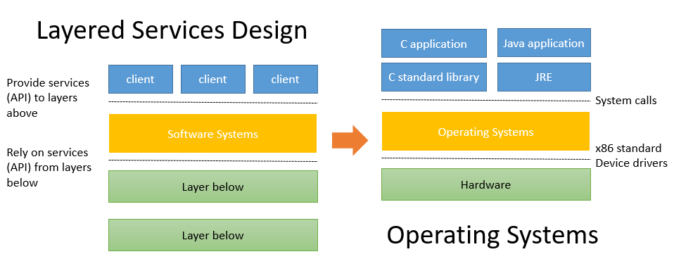
12. Layered Services

• Direct communication between applications and hardware components are impractical due to complexity.
• Operating systems provide much-needed interfaces between applications and hardware through:
  • OS/application interface: system calls.
  • HW/SW interface: x86 standard and device drivers.
• Systems programming: develop software systems that …
  • are composed of multiple modules
  • are complex
  • meets specific requirements in aspects such as performance, security, or fault tolerance.

Key Points

• Computer systems influence the performance and correctness of programs.

Introduction to C

Overview

Teaching: 0 min
Exercises: 0 min

Questions

• How to learn C, once you already not Java?

Objectives

• Know how to write and compile programs in C to a level similar to Java (think at least CSC 142)?

1. What is C?

• Developed by Dennis Ritchie at Bell Labs
• First public released in 1972.
• The book: *The C programming languange” by Dennis M. Ritchie and Brian W. Kernighan. Prentice Hall 1988.

2. How to learn C (now that you already know Java)?

• [C for Java programmers][c4java]
• [C programming vs. Java programming][c_vs_java]

3. Scary stuff ahead …

• C is much less supportive for programmers than Java.
• (Much) easier to make mistake, and (much) harder to fix.

4. But it is exciting …

• C requires less memory resources than Java.
• C, in many instances, runs faster than Java.
• Knowing C will make you a better programmer overall.

5. Similarities (or mostly similar) between C and Java

• Values, types, literals, expressions
• Variables
• Control flow (if, switch, while, for, do-while)
• Call-return: parameters, arguments, return values
• Arrays (mostly)
• Primitive and reference types
• Type casting.
• Library usage.

6. Differences between C and Java

• C has no classes or objects (but something similar)
• C is not object-oriented.
• C arrays are simpler:
  • No boundary checking.
  • No knowledge of array’s own size.
• String operations are limited.
• No collections, exceptions, or generics.
• No automatic memory management.
• Pointers!!!

7. How Java programs run

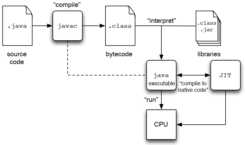
8. How C programs run

9. Hands-on: Getting started

• SSH to molly. Refer to the Setup page if you need a refresher on how to do so.
• Change into csc231 from inside your home directory.
  • Your home directory is represented by the ~ sign.
• Create a directory named intro-c inside csc231, then change into that directory.

$ cd ~/csc231
$ pwd
$ mkdir intro-c
$ ls
$ cd intro-c
$ pwd

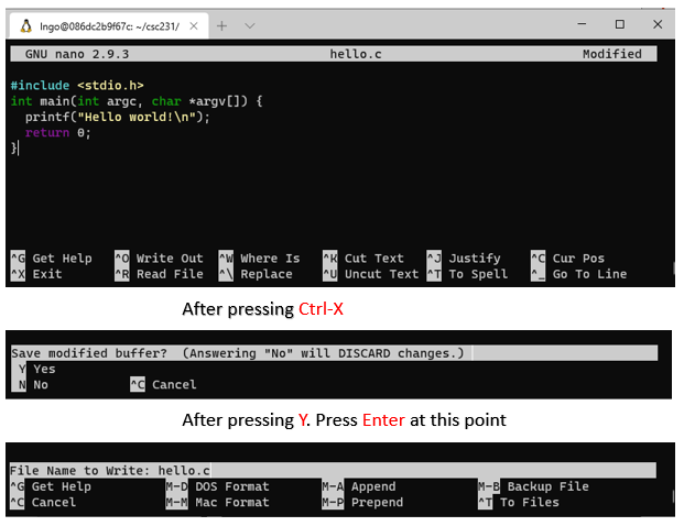
10. Hands-on: Create hello.c

• Inside the terminal, make sure that you are still inside intro-c, then use nano to create hello.cwith the source code below.

$ pwd
$ nano -l hello.c

• Once finished editing in nano:
  • first hit Ctrl-X (same for both Windows and Mac).
  • Next hit Y to save modified buffer (new contents).
  • Hit Enter to save to the same file name as what you opened with.
• Memorize your key-combos!.

What’s in the code?

• Line 1: Standard C library for I/O, similar to Java’s import.
• Line 2-4: Function declaration/definition for main:
  • Line 2:
    • return type: int
    • function name: main
    • parameter list:
      • argc: number of command line arguments.
      • *argv[]: pointers to array of command line argument strings.
  • Line 3: Invoke builtin function printf to print out string Hello world! with an end-of-line character \n. This is similar to System.out.printf.
  • Line 4: Exit a successfully executed program with a return value of 0.

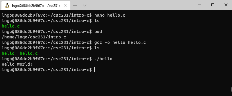
11. Hands-on: Simple compile and run

• Similar to javac, we use gcc to compile C code.
• Before compile, make sure that you are still inside intro-c in the terminal.

$ ls
$ pwd
$ gcc -o hello hello.c
$ ls
$ ./hello

12. Hands-on: Compile and show everything

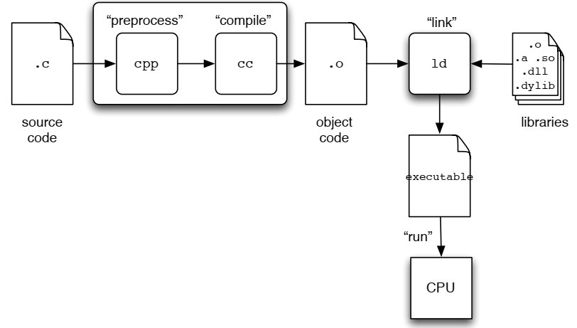
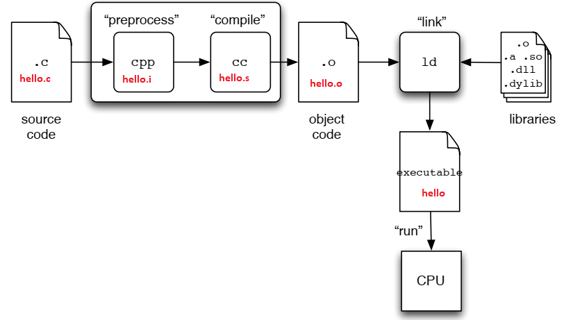
• There are a number of steps from C codes to executable binaries.

$ ls -l
$ gcc -save-temps -o hello2 hello.c
$ ls -l
$ ./hello2

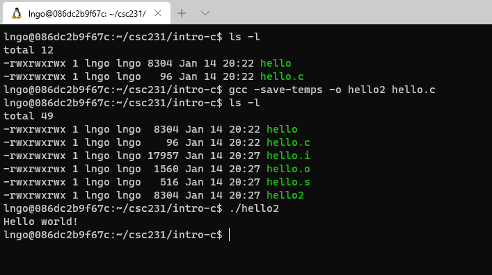
13. What are those?

• hello.i: generated by pre-processor
• hello.s: generated by compiler.
• hello.o: generated by assembler.
• hello (or hello2): executable, generated by linker.

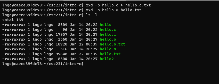
14. Hands-on: View files

• For hello.i and hello.s, they can be view on the editor.
• Run the following command to view hello.i

$ cat -n hello.i

• Run the following command to view hello.s

$ cat -n hello.s

• For hello.o and hello, we need to dump the binary contents first.

$ xxd -b hello.o > hello.o.txt
$ xxd -b hello > hello.txt
$ ls -l

• 

• Run the following command to view hello.o.txt

$ cat -n hello.o.txt

• Run the following command to view hello.txt

$ cat -n hello.txt

15. Challenge:

The usage of C’s printf is similar to Java’s System.out.printf. Find out how to modify hello.c so that the program prints out Hello Golden Rams! with each word on a single line. The program should use exactly one printf statement.

Answer

16. Variables, Addresses, and Pointers

• In Java, you can manipulate the value of a variable via the program but not directly in memory (inside the JVM).
• In C, you can retrieve the address of the location in memory where the variable is stored.
• The operator & (reference of) represents the memory address of a variable.

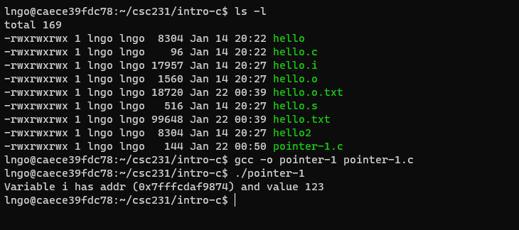
17. Hands-on: Pointer

• Inside the terminal, make suse that you are still inside intro-c, then use nano to create pointer-1.cwith the source code below.

• %p is an output conversion syntax (similar to Java specifiers) for displaying memory address in hex format. See Other Output Conversions for more details.
• Compile and run pointer-1.c

$ ls
$ gcc -o pointer-1 pointer-1.c
$ ./pointer-1

18. Pointer Definition

• Pointer is a variable that points to a memory location (contains a memory location).
  • We can them pointer variables.
• A pointer is denoted by a * character.
• The type of pointer must be the same as that of the value being stored in the memory location (that the pointer points to).
• If a pointer points to a memory location, how do we get these locations?
  • An & character in front of a variable (includes pointer variables) denotes that variable’s address location.

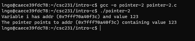
19. Hands-on: Pointer and Variable’s Addresses

• Inside the terminal, make suse that you are still inside intro-c, then use nano to create pointer-2.cwith the source code below.

• Since p_i is a pointer variable, p_i contains a memory address (hence %p).
• Then, *p_i will point to the value in the memory address contained in p_i.
  • This is referred to as de-referencing.
  • This is also why the type of a pointer variable must match the type of data stored in the memory address the pointer variable contains.
• Compile and run pointer-2.c

20. Pass by Value and Pass by Reference

• Parameters are passed to functions.
• Parameters can be value variables or pointer variables.
• What is the difference?

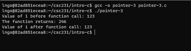
21. Hands-on: Pass by value

• Inside the terminal, make suse that you are still inside intro-c, then use nano to create pointer-3.cwith the source code below.

• Compile and run pointer-3.c

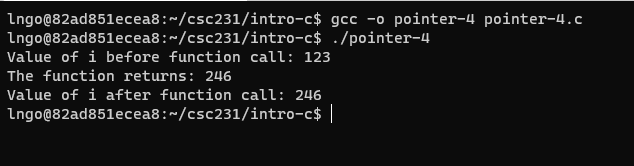
22. Hands-on: Pass by reference

• Inside the terminal, make suse that you are still inside intro-c, then use nano to create pointer-4.cwith the source code below.

• Compile and run pointer-4.c

23. Question

In Java, do you pass by value or pass by reference?

Answer

• Primitives are passed by value.
• Objects are passed by reference.

24. Pointers and memory allocation

• How does C request dynamic memory when you don’t know at compile-time exactly what you will need?
• How does C allocate memory?
  • Automatic: compile arranges for memory to be allocated and initialized for local variables when it is in scope.
  • Static: memory for static variables are allocated once when program starts.
  • Dynamic: memory is allocated on the fly as needed.

25. Dynamic memory allocation

• Unlike Java, you have to do everything!
  • Ask for memory.
  • Return memory when you are done (garbage collection!).
• C function: malloc
  • void *malloc(size_t size);
  • The malloc() function allocates size bytes and returns a pointer to the allocated memory. The memory is not initialized. If size is 0, then malloc() returns either NULL, or a unique pointer value that can later be successfully passed to free().
• C function: free
  • void free(void *ptr);
  • The free() function frees the memory space pointed to by ptr, which must have been returned by a previous call to malloc(), calloc() or realloc(). Otherwise, or if free(ptr) has already been called before, undefined behavior occurs. If ptr is NULL, no operation is performed.

26. Void pointer

• When malloc allocates memory, it returns a sequence of bytes, with no predefined types.
• A pointer that points to this sequence of bytes (the address of the starting byte), is called a void pointer.
• A void pointer will then be typecast to an appropriate type.

27. Hands-on: malloc and type cast

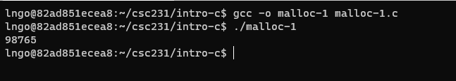
• Inside the terminal, make suse that you are still inside intro-c, then use nano to create malloc-1.cwith the source code below.

• What points to where:
  • void *p = malloc(4);: allocate 4 contiguous bytes. The address of the first byte is returned and assign to pointer variable p. p has no type, so it is a void pointer.
  • int *ip = (int *)p;: The address value pointed to by p is assigned to pointer variable ip. The bytes pointed to be p are now casted to type int.
• Compile and run malloc-1.c

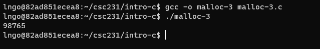
28. Hands-on: malloc and type cast with calculation

• Inside the terminal, make suse that you are still inside intro-c, then use nano to create malloc-2.cwith the source code below.

• Only ask for exactly what you need!
• Compile and run malloc-2.c

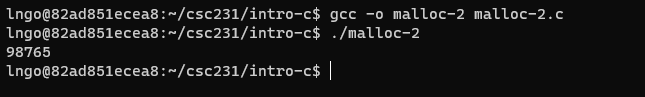
29. Hands-on: Safety

• Inside the terminal, make suse that you are still inside intro-c, then use nano to create malloc-3.cwith the source code below.

• Return and free memory after you are done!
• Compile and run malloc-3.c

30. Dynamic memory allocation

• Critical to support complex data structures that grow as the program executes.
• In Java, custom classes such as ArrayList and Vector provide such support.
• In C, you have to do it manually: How?
• Let’s start with a simpler problem:
  • How can we dynamically allocate memory to an array whose size is not known until during run time?

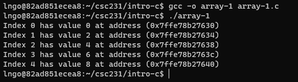
31. Hands-on: What does an array in C look like?

• Inside the terminal, make suse that you are still inside intro-c, then use nano to create array-1.cwith the source code below.

• What is the distance between addresses? Why?
• Compile and run array-1.c

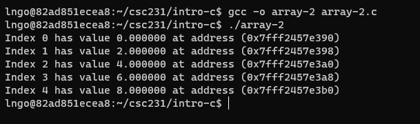
32. Exercise

• Create a copy of array-1.c called array-2.c.
• Change the type of numbers to double.
• What is the address step now?

Answer

33. An array variable

• … is in fact pointing to an address containing a value.
• … without the bracket notation and an index points to the corresponding address of the value at the index.
• … is quite similar to a pointer!

34. Hands-on: Array as pointer (or vice versa …)

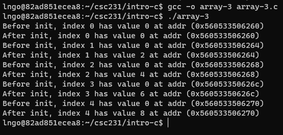
• Inside the terminal, make suse that you are still inside intro-c, then use nano to create array-3.cwith the source code below.

• Compile and run array-3.c

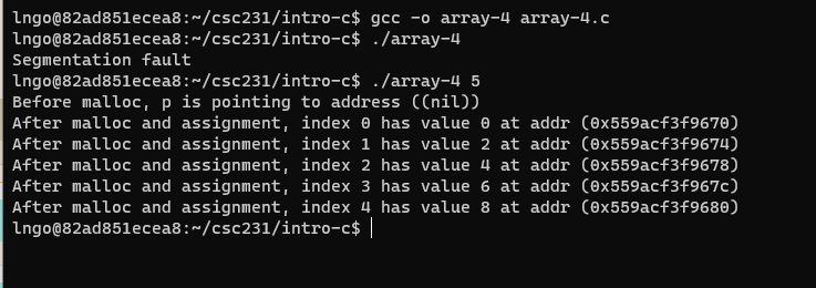
35. Hands-on: Dynamic array creation with command line arguments.

• Inside the terminal, make suse that you are still inside intro-c, then use nano to create array-4.cwith the source code below.

• In C, the command line arguments include the program’s name. The actual arguments start at index position 1 (not 0 like Java).
• Compile and run array-4.c

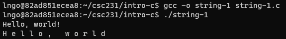
36. Hands-on: String

• Inside the terminal, make suse that you are still inside intro-c, then use nano to create string-1.cwith the source code below.

• Compile and run string-1.c

• In C, string is considered an array of characters.

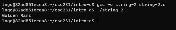
37. Hands-on: Array of strings

• Inside the terminal, make suse that you are still inside intro-c, then use nano to create string-2.cwith the source code below.

• Compile and run string-2.c

38. Object in C

• C has no classes or objects.
• Instead, it has struct type (think ancestor of objects) .

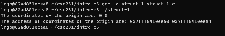
39. Hands-on: Struct in C

• Inside the terminal, make suse that you are still inside intro-c, then use nano to create struct-1.cwith the source code below.

• Compile and run struct-1.c

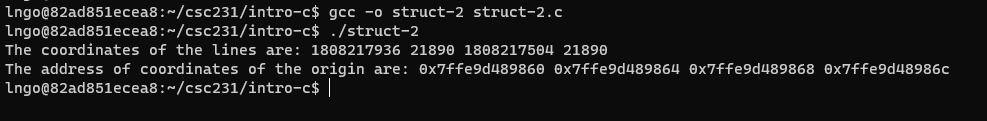
40. Hands-on: Struct of structs in C

• Inside the terminal, make suse that you are still inside intro-c, then use nano to create struct-2.cwith the source code below.

• Compile and run struct-2.c

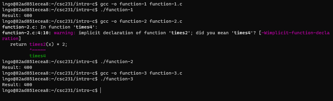
41. Function in C

• Almost the same as methods in Java, except for one small difference.
• They need to either be declared, or must be defined prior to being called (relative to written code position).

42. Hands-on: Functions in C - definition and declaration

• Create three C files, function-1.c, function-2.c, and function-3.c, with the source codes below:

• Compile and run these files.

Key Points

• To learn a new language most efficiently, you are to rely on knowledge from previously known languages.

Representing and manipulating information

Overview

Teaching: 0 min
Exercises: 0 min

Questions

• How do modern computers store and represent information?

Objectives

• Understand different basic bit representation, including two’s complement and floating point representation.

• Understand how bit representations are implemented programmatically in C.

Read chapter 2 of textbook.

1. Everything is bits

• Each bit is 0 or 1
• By encoding/interpreting sets of bits in various ways
  • Computers determine what to do (instructions)
  • … and represent and manipulate numbers, sets, strings, etc…
• Why bits? Electronic Implementation
  • Easy to store with bistable elements.
  • Reliably transmitted on noisy and inaccurate wires.

2. Encoding byte values

• Byte = 8 bits
• Binary: 0000 0000 to 1111 1111.
• Decimal: 0 to 255.
• Hexadecimal: 00 to FF.
  • Base 16 number representation
  • Use character 0 to 9 and A to F.
• Example: 15213 (decimal) = 0011 1011 0110 1101 (binary) = 3B6D (hex)

Hex	0	1	2	3	4	5	6	7	8	9	A	B	C	D	E	F
Decimal	0	1	2	3	4	5	6	7	8	9	10	11	12	13	14	15
Binary	0000	0001	0010	0011	0100	0101	0110	0111	1000	1001	1010	1011	1100	1101	1110	1111

3. Example data representations

C data type	typical 32-bit	typical 64-bit	x86_64
char	1	1	1
short	2	2	2
int	4	4	4
long	4	8	8
float	4	4	4
double	8	8	8
pointer	4	8	8

4. Boolean algebra

• Developed by George Boole in 19th century
• Algebraic representation of logic: encode True as 1 and False as 0.
• Operations: AND (&), OR (|), XOR (^), NOT (~).

A	B	A&B	A|B	A^B	~A
0	0	0	0	0	1
0	1	0	1	1	1
1	0	0	1	1	0
1	1	1	1	0	0

5. General Boolean algebra

• Operate on bit vectors
• Operation applied bitwise.
• All properties of boolean algebra apply.

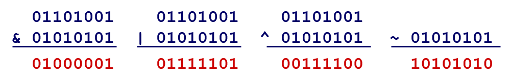
6. Bit-level operations in C

• Boolean operations: &, |, ^, ~.
• Shift operations:
  • Left Shift: x « y
    • Shift bit-vector x left y positions
    • Throw away extra bits on left
    • Fill with 0’s on right
  • Right Shift: x » y
    • Shift bit-vector x right y positions
    • Throw away extra bits on right
    • Logical shift (for unsigned values)
      • Fill with 0’s on left
    • Arithmetic shift (for signed values)
      • Replicate most significant bit on left
  • Undefined Behavior
    • Shift amount < 0 or ≥ word size
• Apply to any “integral” data type: long, int, short, char, unsigned
• View arguments as bit vectors.
• Arguments applied bit-wise.

7. Hands-on: bit-level operations in C

• Open a terminal (Windows Terminal or Mac Terminal).
• Reminder: It is podman on Windows and docker on Mac. Everything else is the same!.
• Launch the container:

Windows:

$ podman run --rm --userns keep-id --cap-add=SYS_PTRACE --security-opt seccomp=unconfined -it -v /mnt/c/csc231:/home/$USER/csc231:Z localhost/csc-container /bin/bash

Mac:

$ docker run --rm --userns=host --cap-add=SYS_PTRACE --security-opt seccomp=unconfined -it -v /Users/$USER/csc231:/home/$USER/csc231:Z csc-container /bin/bash

• Inside your csc231, create another directory called 03-data and change into this directory.
• Create a file named bitwise_demo.c with the following contents:

• Compile and run bitwise_demo.c.
• Confirm that the binary printouts match the corresponding decimal printouts and the expected bitwise operations.

8. Encoding integers

• C does not mandate using 2’s complement.
  • But, most machines do, and we will assume so.

	Decimal	Hex	Binary
short int x	15213	3B 6D	00111011 01101101
short int y	-15213	C4 93	11000100 10010011

• Sign bit
  • For 2’s complement, most significant bit indicates sign.
  • 0 for nonnegative
  • 1 for negative

9. 2’s complement examples

• 2’s complement representation depends on the number of bits.
• Technical trick: A binary representation of the absolute value of negative 2 to the power of the number of bits minus the absolute value of the negative number.
• Simple example for 5-bit representation

	-16	8	4	2	1
10	0	1	0	1	0	8 + 2 = 10
-10	1	0	1	1	0	-16 + 4 + 2 = -10

• Simple example for 6-bit representation

	-32	16	8	4	2	1
10	0	0	1	0	1	0	8 + 2 = 10
-10	1	1	0	1	1	0	-32 + 16 + 4 + 2 = -10

• Complex example

	Decimal	Hex	Binary
short int x	15213	3B 6D	00111011 01101101
short int y	-15213	C4 93	11000100 10010011

Weight	15213		-15213
1	1	1	1	1
2	0	0	1	2
4	1	4	0	0
8	1	8	0	0
16	0	0	1	16
32	1	32	0	0
64	1	64	0	0
128	0	0	1	128
256	1	256	0	0
512	1	512	0	0
1024	0	0	1	1024
2048	1	2048	0	0
4096	1	4096	0	0
8192	1	8192	0	0
16384	0	0	1	16384
-32768	0	0	1	-32768
Sum		15213		-15213

10. Numeric ranges

• Unsigned values for w-bit word
  • UMin = 0
  • UMax = 2^w - 1
• 2’s complement values for w-bit word
  • TMin = -2^w-1
  • TMax = 2^w-1 - 1
  • -1: 111..1
• Values for different word sizes:

	8 (1 byte)	16 (2 bytes)	32 (4 bytes)	64 (8 bytes)
UMax	255	65,535	4,294,967,295	18,446,744,073,709,551,615
TMax	127	32,767	2,147,483,647	9,223,372,036,854,775,807
TMin	-128	-32,768	-2,147,483,648	-9,223,372,036,854,775,808

• Observations
  • abs(TMin) = TMax + 1
    • Asymetric range
  • UMax = 2 * TMax + 1
• C programming
  • #include <limits.h>
  • Declares constants: ULONG_MAX, LONG_MAX, LONG_MIN
  • Platform specific

11. Challenge

• Write a C program called numeric_ranges.c that prints out the value of ULONG_MAX, LONG_MAX, LONG_MIN. Also answer the following question: If we multiply LONG_MIN by -1, what do we get?
• Note: You need to search for the correct format string specifiers.

Solution

12. Conversions (casting)

• C allows casting between different numeric data types.
• What should be the effect/impact?
• Notations:
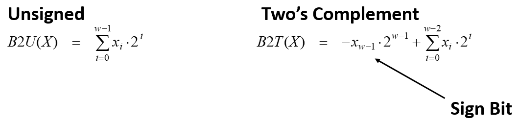
  • B2T: Binary to 2’s complement
  • B2U: Binary to unsigned
  • U2B: Unsigned to binary
  • U2T: Usigned to 2’s complement
  • T2B: 2’s complement to binary
  • T2U: 2’s complement to unsigned

13. Visualization of conversions

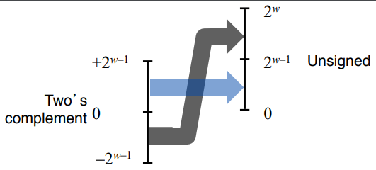
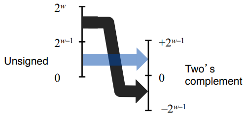
• T2U_w(x) = x + 2^w if x < 0
• T2U_w(x) = x if x >= 0

• U2T_w(x) = x - 2^w if x > TMax_w

• U2T_w(x) = x if x <= TMax_w

• Summary
  • Bit pattern is maintained but reinterpreted
  • Can have unexpected effects: adding or subtracting 2^w
  • When expressions contain both signed and unsigned int values, int values will be casted to unsigned.

14. Hands on: casting

• Make sure that you are inside 03-data directory.
• Create a file named casting.c with the following contents:

• Compile and run casting.c.
• Confirm that converted values are correct based on equations from slide 13.

15. Challenge

• What is wrong with the following program?
• How can this program be corrected?

Solution

16. Expanding and truncation

• Expanding (e.g., short int to int)
  • Unsigned: zeros added
  • Signed: sign extension
  • Both yield expected result

• Truncating (e.g., unsigned to unsigned short)
  • Unsigned/signed: bits are truncated
  • Result reinterpreted
  • Unsigned: mod operation
  • Signed: similar to mod
  • For small (in magnitude) numbers yields expected behavior

17. Misunderstanding integers can lead to the end of the world!

• Thule Site J: USAF radar station for missile warning and spacecraft tracking.
• “There are many examples of errors arising from incorrect or incomplete specifications. One such example is a false alert in the early days of the nuclear age, when on October 5, 1960, the warning system at NORAD indicated that the United States was under massive attack by Soviet missiles with a certainty of 99.9 percent. It turned out that the Ballistic Missile Early Warning System (BMEWS) radar in Thule, Greenland, had spotted the rising moon. Nobody had thought about the moon when specifying how the system should act.” (Computer System Reliability and Nuclear War, CACM 1987).
• Moon’s large size: 1000s of objects reported.
• Moon’s distance: .25 million miles
  • Thule’s BMEWS max distance: 3000 miles.
  • Truncated distance to the moon: % sizeof(distance) = 2200 miles.
• Remember assignment 1: The computer does not “see”, it only interprets.
  • Thousands of objects on the sky within missile detection range!.
• Human control:
  • Kruschev was in New York on October 5, 1960.
  • Someone at Thule said, “why not go check outside?”

18. Unsigned addition

• Given w bits operands
• True sum can have w + 1 bits (carry bit).
• Carry bit is discarded.
• Implementation:
• s = (u + v) mod 2^w

19. Hands on: unsigned addition

• Make sure that you are inside 03-data directory.
• Create a file named unsigned_addition.c with the following contents:

• Compile and run unsigned_addition.c.
• Confirm that calculated values are correct.

20. 2’s complement addition

• Almost similar bit-level behavior as unsigned addition
  • True sum of w-bit operands will have w+1-bit, but
  • Carry bit is discarded.
  • Remainding bits are treated as 2’s complement integers.
• Overflow behavior is different
• TAdd_w(u, v) = u + v + 2^w if u + v < TMin_w (Negative Overflow)
• TAdd_w(u, v) = u + v if TMin_w <= u + v <= TMax_w
• TAdd_w(u, v) = u + v - 2^w if u + v > TMax_w (Positive Overflow)

21. Hands on: signed addition

• Make sure that you are inside 03-data directory.
• Create a file named signed_addition.c with the following contents:

• Compile and run signed_addition.c.
• Confirm that calculated values are correct.

22. Multiplication

• Compute product of w-bit numbers x and y.
• Exact results can be bigger than w bits.
  • Unsigned: up to 2w bits: 0 <= x * y <= (2^w - 1)²
  • 2’s complement (negative): up to 2w - 1 bits: x * y >= (-2)^2w-2 + 2^2w-1
  • 2’s complement (positive): up to 2w bits: x * y <= 2^2w-2
• To maintain exact results:
  • Need to keep expanding word size with each product computed.
  • Is done by software if needed (arbitrary precision arithmetic packages).
• Trust your compiler: Modern CPUs and OSes will most likely know to select the optimal method to multiply.

23. Multiplication and Division by power-of-2

• Power-of-2 multiply with shift
  • u >> k gives u * 2^k
  • True product has w + k bits: discard k bits.
• Unsigned power-of-2 divide with shift
  • u >> k gives floor(u / 2^k)
  • Use logical shift.
• Signed power-of-2 divide with shift
  • x > 0: x >> k gives floor(u / 2^k)
  • x < 0: (x + (1 << k) - 1) >> k gives ceiling(u / 2^k)
  • C statement: (x < 0 ? x + (1 << k) - 1: x) >> k

24. Negation: complement and increase

• Negate through complement and increment:
  • ~x + 1 == -x

25. Challenge

• Implement a C program called negation.c that implements and validates the equation in slide 24. The program should take in a command line argument that takes in a number of type short to be negated.
• What happens if you try to negate -32768?

Solution

26. Byte-oriented memory organization

• Programs refer to data by address
  • Conceptually, envision it as a very large array of bytes
    • In reality, it’s not, but can think of it that way
  • An address is like an index into that array
    • and, a pointer variable stores an address
• Note: system provides private address spaces to each “process”
  • Think of a process as a program being executed
  • So, a program can clobber its own data, but not that of others

27. Machine words

• Any given computer has a “Word Size”
• `word size”: Nominal size of integer-valued data and of addresses
• Until recently, most machines used 32 bits (4 bytes) as word size
  • Limits addresses to 4GB (232 bytes)
• Increasingly, machines have 64-bit word size
  • Potentially, could have 18 EB (exabytes) of addressable memory
  • That’s 18.4 X 1018
• Machines still support multiple data formats
  • Fractions or multiples of word size
  • Always integral number of bytes

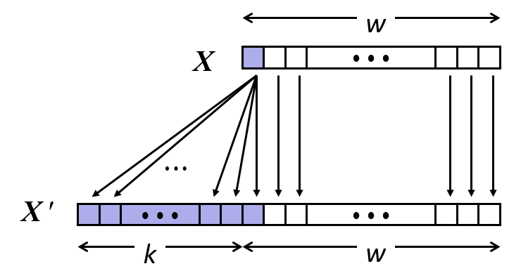
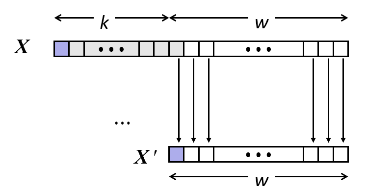
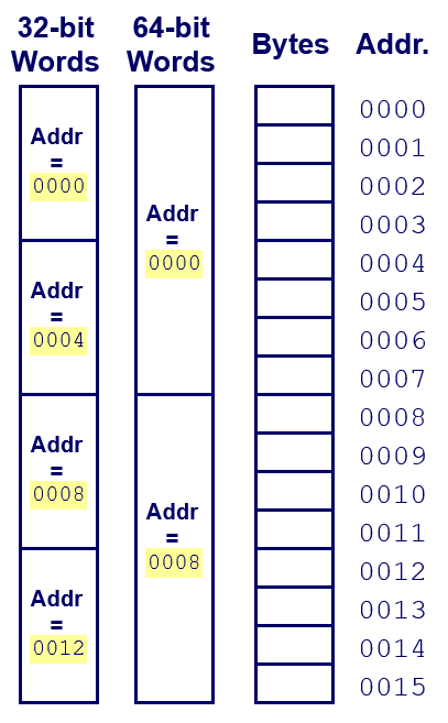
28. Word-oriented memory organization

• Addresses specific byte locations
  • Address of first byte in word.
  • Address of successive words differ by 4 (32-bit) or 8 (64-bit).

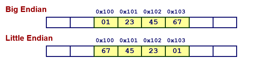
30. Byte ordering in memory

• Machine-dependent
• Big Endian: Sun (Oracle SPARC), PPC Mac, Internet (network data transfer)
  • Least significant byte has the highest address.
• Little Endian: x86, ARM processors running Android, iOS, and Linux
  • Least significant byte has lowest address.
• Example
  • Variable x has 4-byte value of 0x01234567
  • Address given by &x is 0x100

31. Hands on: byte ordering in memory

• Make sure that you are inside 03-data directory.
• Create a file named byte_ordering.c with the following contents:

• Compile and run byte_ordering.c.
• Confirm that calculated values are correct.

32. Fractional binary numbers

• What is 1011.101₂?
  • 8 + 0 + 2 + 1 + 1/2 + 0 + 1/4
• Can only exactly represent numbers of the form x/2^k
• Limited range of numbers within the w-bit word size.

33. IEEE Foating point

• IEEE Standard 754
  • Established in 185 as uniform standard for floating point arithmetic
  • Supported by all major CPUs
  • Some CPUs don’t implement IEEE 754 in full, for example, early GPUs, Cell BE processor
• Driven by numerical concerns
  • Nice standards for rounding, overflow, underflow
  • Hard to make fast in hardware (Numerical analysts predominated over hardware designers in defining standard).

34. Importance of floating-point arithmetic accuracy

• Ariane 5 explordes on maiden voyage: $500 million dollars lost.
  • 64-bit floating point number assigned to 16-bit integer
  • Cause rocket to get incorrect value of horizontal velocity and crash.
• Patriot Missle defense system misses Scud: 28 dead
  • Velocity is a real number that can be expressed as a whole number and a decimal (e.g., 3750.2563…miles per hour). Time is kept continuously by the system’s internal clock in tenths of seconds but is expressed as an integer or whole number (e.g., 32,33, 34…). The longer the system has been running, the larger the number representing time. To predict where the Scud will next appear, both time and velocity must be expressed as real numbers. Because of the way the Patriot computer performs its calculations and the fact that its registers are only 24 bits long, the conversion of time from an integer to a real number cannot be any more precise than 24 bits. This conversion results in a loss of precision causing a less accurate time calculation. The effect of this inaccuracy on the range gate’s calculation is directly proportional to the target’s velocity and the length of time the system has been running. Consequently, performing the conversion after the Patriot has been running continuously for extended periods causes the range gate to shift away from the center of the target, making it less likely that the target, in this case a Scud, will be successfully intercepted.

35. IEEE Foating point representation

• Numerical form: (-1)^sM2^E
  • Sign bit s determins whether the number is negative or positive.
  • Significantd M normalizes a fractional value in range [1.0, 2.0).
  • Exponent E weights value by power of two.
• Encoding
  • Most significant bit is sign bit s.
  • exp field encodes E (but is not equal to E)
  • frac field encodes M (but is not equalt to M)

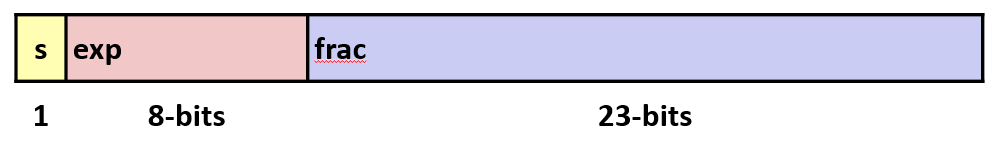
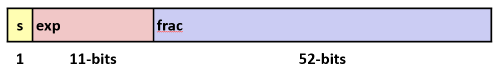
• Single precision: 32 bits

• Double precision: 64 bits

36. Three “kinds” of floating point numbers

• Depends on the exp field (E).
• Denormalized: exp contains all 0s.
• Special: exp contains all 1s.
• Normalized: exp contains a mix of 0s and 1s.

37. Normalized floating point numbers

• When: exp != 000…0 and exp != 111…1
• Exponent coded as a biased value: E = exp – Bias
  • exp: unsigned value of exp field
  • Bias = 2^k-1 - 1, where k is number of exponent bits
    • Single precision: 127 (exp: 1…254, E: -126…127)
    • Double precision: 1023 (exp: 1…2046, E: -1022…1023)
• Significand coded with implied leading 1: M = 1.xxx…x₂
  • xxx…x: bits of frac field
  • Minimum when frac=000…0 (M = 1.0)
  • Maximum when frac=111…1 (M = 2.0 – ε)
  • Get extra leading bit for “free” (hence the range: [1.0, 2.0))

38. Example: normalized floating point numbers

• Value: float F = 15213.0;
  • 15213₁₀ = 11101101101101₂ = 1.1101101101101₂ * 2¹³
• Significand:
  • M = 1.1101101101101₂
  • frac = 11011011011010000000000₂
• Exponent:
  • E = 13
  • Bias = 127
  • exp = 140 = 10001100₂

• Result: 0

  10001100

  11011011011010000000000

39. Hands on: check floating point representation

• Make sure that you are inside 03-data directory.
• Create a file named show_fp.c with the following contents:

• Compile and run show_fp.c.
• Confirm that calculated values in slide 38 are correct.

40. Denormalized floating point

• Condition: exp = 000…0
• Exponent value: E = 1 – Bias
• Significand coded with implied leading 0: M = 0.xxx…x₂
  • xxx…x: bits of frac
• Cases
  • exp = 000…0, frac = 000…0
    • Represents zero value
    • Note distinct values: +0 and –0
  • exp = 000…0, frac ≠ 000…0
    • Numbers closest to 0.0
    • Equispaced

41. Special cases

• Condition: exp = 111…1
• Case: exp = 111…1, frac = 000…0
  • Represents value infinity
  • Operation that overflows
  • Both positive and negative
• Case: exp = 111…1, frac != 000…0
  • Not-a-Number (NaN)
  • Represents case when no numeric value can be determined

42. Floating operations: basic idea

• Compute exact result.
• Make it fit into desired precision.
  • Possible overflow if exponent too large
  • Possible round to fit into frac
• Rounding modes

	1.40	1.60	1.50	2.50	-1.50
Towards zero	1	1	1	2	-1
Round down	1	1	1	2	-2
Round up	2	1	1	3	-1
Nearest even (default)	1	2	2	2	-2

• Nearest even
  • Hard to get any other mode without dropping into assembly.
  • C99 has support for rounding mode management
• All others are statistically based
  • Sum of set of positive numbers will consistently be over- or under-estimated.

43. Floating point multiplication

• (-1)^s₁M₁2^E₁ * (-1)^s₂M₂2^E₂.
• Exact result: (-1)^sM2^E
  • s = s₁^s₂
  • M = M₁*M₂
  • E = E₁+E₂
• Correction
  • If M >= 2, shift M right, increment E.
  • If E out of range, overflow.
  • Round M to fit frac precision
• Implementation: Biggest chore is multiplying significands.

44. Floating point addition

• (-1)^s₁M₁2^E₁ + (-1)^s₂M₂2^E₂.
• Exact result: (-1)^sM2^E
  • Sign s, significand M: result of signed align and add
  • E = E₁
• Correction
  • If M >= 2, shift M right, increment E.
  • If M < 1, shift M left k positions, decrement E by k.
  • Overflow if E out of range
  • Round M to fit frac precision
• Implementation: Biggest chore is multiplying significands.

45. Mathematical properties of floating point addition

• Compare to those of Abelian group (a group in which the result of applying the group operation to two group elements does not depend on the order in which they are written):
  • Closed under addition? Yes (but may generate infinity or NaN)
  • Communicative? Yes
  • Associative? No
    • Overflow and inexactness of rounding
    • (3.14+1e10)-1e10 = 0, 3.14+(1e10-1e10) = 3.14
  • 0 is additive identity? Yes
  • Every elemtn has additive inverse? Almost
    • Except for infinities and NaN
• Monotonicity?
  • Almost
  • Except for infinities and NaN

46. Mathematical properties of floating point multiplication

• Compare to those of Abelian group (a group in which the result of applying the group operation to two group elements does not depend on the order in which they are written):
  • Closed under addition? Yes (but may generate infinity or NaN)
  • Communicative? Yes
  • Associative? No
    • Overflow and inexactness of rounding
    • (1e20 * 1e20) * 1e-20= inf, 1e20 * (1e20 * 1e-20)= 1e20
  • 1 is additive identity? Yes
  • Multiplication distributes over addition? No
    • Overflow and inexactness of rounding
    • 1e20 * (1e20-1e20)= 0.0, 1e20 * 1e20 – 1e20 * 1e20 = NaN
• Monotonicity?
  • Almost
  • Except for infinities and NaN

47. Floating point in C

• C guarantees two levels
  • float: single precision
  • double: double precision
• Conversion/casting
  • Casting between int, float, and double changes bit representation
  • double/float to int
    • Truncates fractional part
    • Like rounding toward zero
    • Not defined when out of range or NaN: Generally sets to TMin
  • int to double
    • Exact conversion, as long as int has ≤ 53 bit word size
  • int to float
    • Will round according to rounding mode

Key Points

• Various information representation schemes are utilized to represent different data types given the bit-size limitations.

Machine language and debugging

Overview

Teaching: 0 min
Exercises: 0 min

Questions

• Getting closer to the hardware via machine languages

Objectives

• First learning objective. (FIXME)

1. Intel x86 processors

• Dominate laptop/desktop/server market
• Evolutionary design
  • Backwards compatible up until 8086, introduced in 1978
  • Added more features as time goes on
• x86 is a Complex Instruction Set Computer (CISC)
  • Many different instructions with many different formats
  • But, only small subset encountered with Linux programs
• Compare: Reduced Instruction Set Computer (RISC)
  • RISC: very few instructions, with very few modes for each
  • RISC can be quite fast (but Intel still wins on speed!)
  • Current RISC renaissance (e.g., ARM, RISC V), especially for low-power

2. Intel x86 processors: machine evolution

Name	Date	Transistor Counts
386	1985	0.3M
Pentium	1993	3.1M
Pentium/MMX	1997	4.5M
Pentium Pro	1995	6.5M
Pentium III	1999	8.2M
Pentium 4	2000	42M
Core 2 Duo	2006	291M
Core i7	2000	42M
Core i7 Skylake	2006	291M

• Added features
  • Instructions to support multimedia operations
  • Instructions to enable more efficient conditional operations (!)
  • Transition from 32 bits to 64 bits
  • More cores

3. x86 clones: Advanced Micro Devices (AMD)

• Historically
  • AMD has followed just behind Intel
  • A little bit slower, a lot cheaper
• Then
  • Recruited top circuit designers from Digital Equipment Corp. and other downward trending companies
  • Built Opteron: tough competitor to Pentium 4
  • Developed x86-64, their own extension to 64 bits
• Recent Years
  • Intel got its act together
    • 1995-2011: Lead semiconductor “fab” in world
    • 2018: #2 largest by $$ (#1 is Samsung)
    • 2019: reclaimed #1
• AMD fell behind
  • Relies on external semiconductor manufacturer GlobalFoundaries
  • ca. 2019 CPUs (e.g., Ryzen) are competitive again
  • 2020 Epyc

4. Machine programming: levels of abstraction

• Architecture: (also ISA: instruction set architecture) The parts of a processor design that one needs to understand for writing correct machine/assembly code
  • Examples: instruction set specification, registers
  • Machine Code: The byte-level programs that a processor executes
  • Assembly Code: A text representation of machine code
• Microarchitecture: Implementation of the architecture
  • Examples: cache sizes and core frequency
• Example ISAs:
  • Intel: x86, IA32, Itanium, x86-64
  • ARM: Used in almost all mobile phones
  • RISC V: New open-source ISA

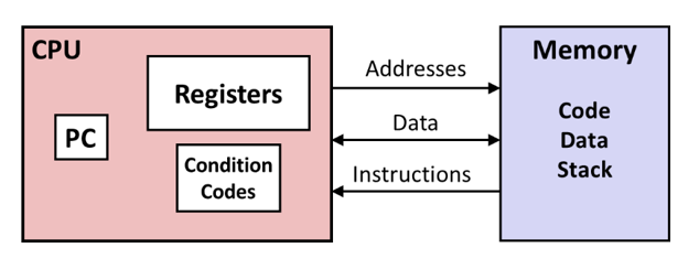
5. Assembly/Machine code view

• Machine code (Assembly code) differs greatly from the original C code.
• Parts of processor state that are not visible/accessible from C programs are now visible.
  • PC: Program counter
    • Contains address of next instruction
    • Called %rip (instruction pointer register)
  • Register file
    • contains 16 named locations (registers), each can store 64-bit values.
    • These registers can hold addresses (~ C pointers) or integer data.
  • Condition codes
    • Store status information about most recent arithmetic or logical operation
    • Used for conditional branching (if/while)
  • Vector registers to hold one or more integers or floating-point values.
  • Memory
    • Is seen as a byte-addressable array
    • Contains code and user data
    • Stack to support procedures

6. Hands on: assembly/machine code example

• Open a terminal (Windows Terminal or Mac Terminal).
• Reminder: It is podman on Windows and docker on Mac. Everything else is the same!.
• Launch the container:

Windows:

$ podman run --rm --userns keep-id --cap-add=SYS_PTRACE --security-opt seccomp=unconfined -it -v /mnt/c/csc231:/home/$USER/csc231:Z localhost/csc-container /bin/bash

Mac:

$ docker run --rm --userns=host --cap-add=SYS_PTRACE --security-opt seccomp=unconfined -it -v /Users/$USER/csc231:/home/$USER/csc231:Z csc-container /bin/bash

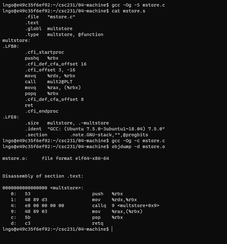
• Inside your csc231, create another directory called 04-machine and change into this directory.
• Create a file named mstore.c with the following contents:

• Run the following commands It is capital o, not number 0

$ gcc -Og -S mstore.c
$ cat mstore.s
$ gcc -Og -c mstore.c
$ objdump -d mstore.o

• x86_64 instructions range in length from 1 to 15 bytes
• The disassembler determines the assembly code based purely on the byte-sequence in the machine-code file.
• All lines begin with . are directirves to the assembler and linker.

7. Data format

C data type	Intel data type	Assembly-code suffix	Size
char	Byte	b	1
short	Word	w	2
int	Double word	l	4
long	Quad word	q	8
char *	Quad word	q	8
float	Single precision	s	4
double	Double precision	l	8

8. Integer registers

• x86_64 CPU contains a set of 16 general purpose registers storing 64-bit values.
• Original 8086 design has eight 16-bit registers, %ax through %sp.
  • Origin (mostly obsolete)
    • %ax: accumulate
    • %cx: counter
    • %dx: data
    • %bx: base
    • %si: source index
    • %di: destination index
    • %sp: stack pointer
    • %bp: base pointer
• After IA32 extension, these registers grew to 32 bits, labeled %eax through %esp.
• After x86_64 extension, these registers were expanded to 64 bits, labeled %rax through %rsp. Eight new registered were added: %r8 through %r15.
• Instructions can operate on data of different sizes stored in low-order bytes of the 16 registers.

Bryant and O’ Hallaron, Computer Systems: A Programmer’s Perspective, Third Edition

9. Assembly characteristics: operations

• Transfer data between memory and register
  • Load data from memory into register
  • Store register data into memory
• Perform arithmetic function on register or memory data
• Transfer control
  • Unconditional jumps to/from procedures
  • Conditional branches
  • Indirect branches

10. Data movement

• Example: movq Source, Dest
• Note: This is ATT notation. Intel uses mov Dest, Source
• Operand Types:
  • Immediate (Imm): Constant integer data.
    • $0x400, $-533.
    • Like C constant, but prefixed with $.
    • Encoded with 1, 2, or 4 bytes.
  • Register (Reg): One of 16 integer registers
    • Example: %rax, %r13
    • %rsp reserved for special use.
    • Others have special uses in particular instructions.
  • Memory (Mem): 8 (q in movq) consecutive bytes of memory at address given by register.
    • Example: (%rax)
    • Various other addressing mode (See textbook page 181, Figure 3.3).
• Other mov:
  • movb: move byte
  • movw: move word
  • movl: move double word
  • movq: move quad word
  • moveabsq: move absolute quad word

11. movq Operand Combinations

movq	Source	Dest	Src, Dest	C Analog
	Imm	Reg	movq $0x4, %rax	tmp = 0x4;
	Imm	Mem	movq $-147,(%rax)	*p = -147;
	Reg	Reg	movq %rax,%rdx	tmp2 = tmp1;
	Reg	Mem	movq %rax,(%rdx)	*p = tmp;
	Mem	Reg	movq (%rax),%rdx	tmp = *p;

12. Simple memory addressing mode

• Normal: (R) Mem[Reg[R]]
  • Register R specifies memory address
  • Aha! Pointer dereferencing in C
  • movq (%rcx),%rax
• Displacement D(R) Mem[Reg[R]+D]
  • Register R specifies start of memory region
  • Constant displacement D specifies offset
  • movq 8(%rbp),%rdx

13. x86_64 Cheatsheet

Brown University - Dr. Doeppner

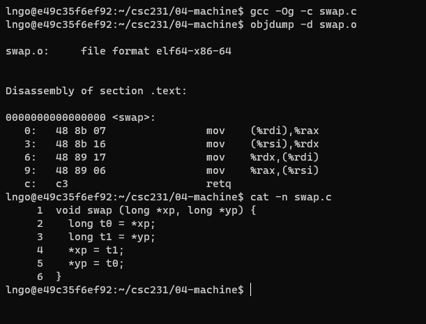
14. Hands on: data movement

• Create a file named swap.c in 04-machine with the following contents:

• Run the following commands

$ gcc -Og -c swap.c
$ objdump -d swap.o

• Why %rsi and %rdi?
• Procedure Data Flow:
  • First six parameters will be placed into rdi, rsi, rdx, rcx, r8, r9.
  • The remaining parameters will be pushed on to the stack of the calling function.

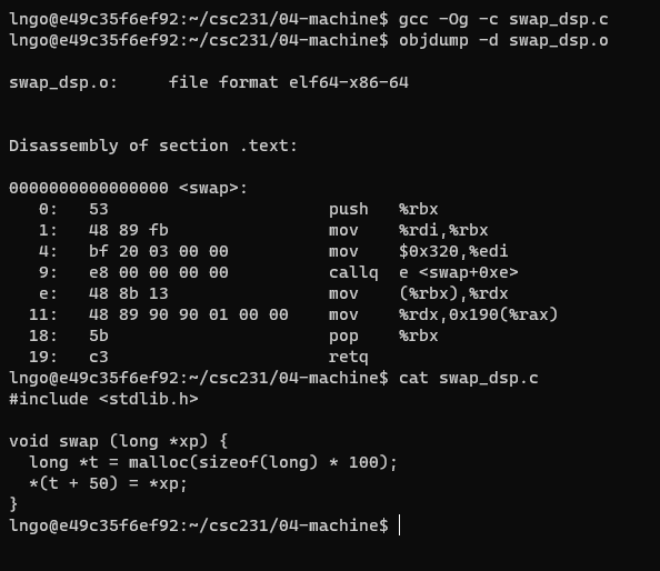
15. Hands on: data movement

• Create a file named swap_dsp.c in 04-machine with the following contents:

• Run the following commands

$ gcc -Og -c swap_dsp.c
$ objdump -d swap_dsp.o

• What is the meaning of 0x190?

16. Complete memory addressing mode

• Most General Form
  • D(Rb,Ri,S): Mem[Reg[Rb]+S*Reg[Ri]+ D]
  • D: Constant displacement 1, 2, or 4 bytes
  • Rb: Base register: Any of 16 integer registers
  • Ri: Index register: Any, except for %rsp
  • S: Scale: 1, 2, 4, or 8
• Special Cases
  • (Rb,Ri): Mem[Reg[Rb]+Reg[Ri]]
  • D(Rb,Ri): Mem[Reg[Rb]+Reg[Ri]+D]
  • (Rb,Ri,S): Mem[Reg[Rb]+S*Reg[Ri]]
  • (,Ri,S): Mem[S*Reg[Ri]]
  • D(,Ri,S): Mem[S*Reg[Ri] + D]

17. Arithmetic and logical operations: lea

• lea: load effective address
• A form of movq intsruction
  • lea S, D: Write &S to D.
  • can be used to generate pointers
  • can also be used to describe common arithmetic operations.

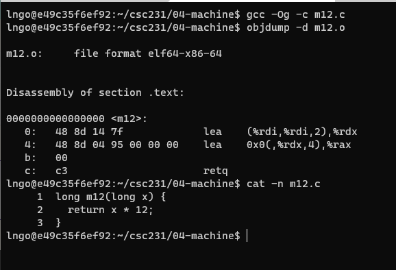
18. Hands on: lea

• Create a file named m12.c in 04-machine with the following contents:

• Run the following commands

$ gcc -Og -c m12.c
$ objdump -d m12.o

• Review slide 16
• %rdi: x
• (%rdi, %rdi,2) = x + 2 * x
• The above result is moved to %rdx with lea.
• 0x0(,%rdx,4) = 4 * (x + 2 * x) = 12*x
• The above result is moved to %rax with lea.

19. Other arithmetic operations

• Omitting suffixes comparing to the book.

Format	Computation	Description
add Src,Dest	D <- D + S	add
sub Src,Dest	D <- D - S	subtract
imul Src,Dest	D <- D * S	multiply
shl Src,Dest	D <- D « S	shift left
sar Src,Dest	D <- D » S	arith. shift right
shr Src,Dest	D <- D » S	shift right
sal Src,Dest	D <- D « S	arith. shift left
xor Src,Dest	D <- D ^ S	exclusive or
and Src,Dest	D <- D & S	and
or Src,Dest	D <- D | S	or
inc Src	D <- D + 1	increment
dec Src	D <- D - 1	decrement
neg Src	D <- -D	negate
not Src	D <- -D	complement

• Watch out for argument order (ATT versus Intel)
• No distinction between signed and unsigned int. Why is that?

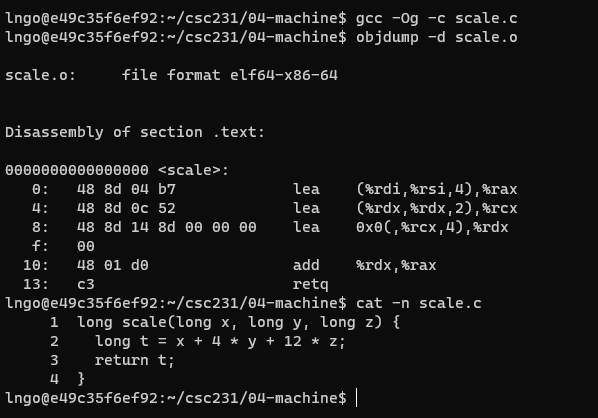
20. Challenge: lea

• Create a file named scale.c in 04-machine with the following contents:

• Run the following commands

$ gcc -Og -c scale.c
$ objdump -d scale.o

• Identify the registers holding x, y, and z.
• Which register contains the final return value?

Solution

• %rdi: x
• %rsi: y
• %rdx: z
• %rax contains the final return value.

Midterm

• Friday April 2, 2021
• 24-hour windows range: 12:00AM - 11:59PM April 2, 2021.
• 75 minutes duration.
• 20 questions (similar in format to the quizzes).
• Everything (including source codes) up to slide 20 of Machine language and debugging.
• No class on Friday April 2.

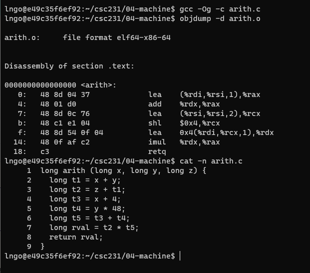
21. Hands on: long arithmetic

• Create a file named arith.c in 04-machine with the following contents:

• Run the following commands

$ gcc -Og -c arith.c
$ objdump -d arith.o

• Understand how the Assembly code represents the actual arithmetic operation in the C code.

22. Quick review: processor state

• Information about currently executing program
  • temporary data (%rax,…)
  • location of runtime stack (%rsp)
  • location of current code control point (%rip,…)
  • status of recent tests (CF, ZF, SF, OF in %EFLAGS)

23. Condition codes (implicit setting)

• Single-bit registers
  • CF: the most recent operation generated a carry out of the most significant bit.
  • ZF: the most recent operation yielded zero.
  • SF: the most recent operation yielded negative.
  • OF: the most recent operation caused a two’s-complement overflow.
• Implicitly set (as side effect) of arithmetic operations.

24. Condition codes (explicit setting)

• Exlicit setting by Compare instruction
  • cmpq Src2, Src1
  • cmpq b, a like computing a - b without setting destination
• CF set if carry/borrow out from most significant bit (unsigned comparisons)
• ZF set if a == b
• SF set if (a - b) < 0
• OF set if two’s complement (signed) overflow
  • (a>0 && b<0 && (a-b)<0) || (a<0 && b>0 && (a-b)>0)

25. Condition branches (jX)

• Jump to different part of code depending on condition codes
• Implicit reading of condition codes

jX	Condition	Description
jmp	1	direct jump
je	ZF	equal/zero
jne	~ZF	not equal/not zero
js	SF	negative
jns	~SF	non-negative
jg	~(SF^OF) & ~ZF	greater
jge	~(SF^OF)	greater or equal to
jl	SF^OF	lesser
jle	SF^OF | ZF	lesser or equal to
ja	~CF & ~ZF	above
jb	CF	below

26. Hands on: a simple jump

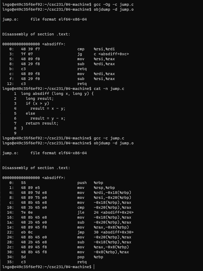
• Create a file named jump.c in 04-machine with the following contents:

• Run the following commands

$ gcc -Og -c jump.c
$ objdump -d jump.o

• Understand how the Assembly code enables jump across instructions to support conditional workflow.

• Rerun the above commands but ommit -Og flag. Think about the differences in the resulting Assembly code.

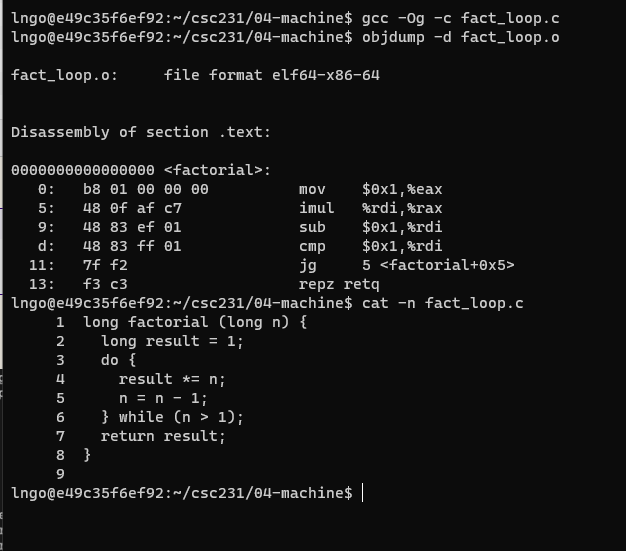
27. Hands on: loop

• Create a file named fact_loop.c in 04-machine with the following contents:

• Run the following commands

$ gcc -Og -c fact_loop.c
$ objdump -d fact_loop.o

• Understand how the Assembly code enables jump across instructions to support loop.

• Create fact_loop_2.c and fact_loop_3.c from fact_loop.c.
• Modify fact_loop_2.c so that the factorial is implemented with a while loop. Study the resulting Assembly code.
• Modify fact_loop_3.c so that the factorial is implemented with a for loop. Study the resulting Assembly code.

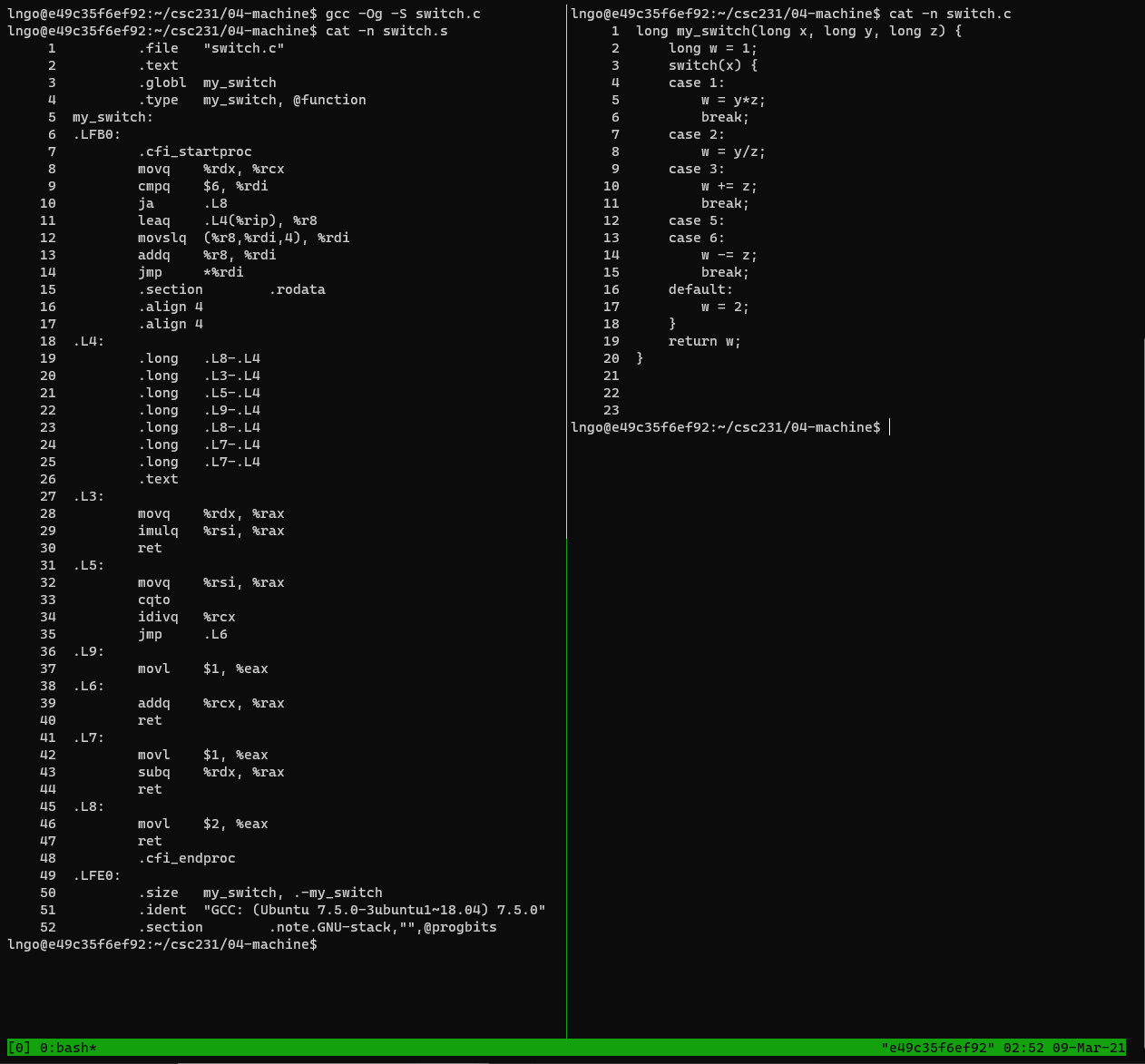
28. Hands on: switch

• Create a file named switch.c in 04-machine with the following contents:

• View switch.c and the resulting switch.s in a two-column tmux terminal.

$ gcc -Og -S switch.c

29. Mechanisms in procedures

• Function = procedure (book terminology)
• Support procedure P calls procedure Q.
• Passing control
  • To beginning of procedure code
    • starting instruction of Q
  • Back to return point
    • next instruction in P after Q
• Passing data
  • Procedure arguments
    • P passes one or more parameters to Q.
    • Q returns a value back to P.
  • Return value
• Memory management
  • Allocate during procedure execution and de-allocate upon return
    • Q needs to allocate space for local variables and free that storage once finishes.
• Mechanisms all implemented with machine instructions
• x86-64 implementation of a procedure uses only those mechanisms required
• Machine instructions implement the mechanisms, but the choices are determined by designers. These choices make up the Application Binary Interface (ABI).

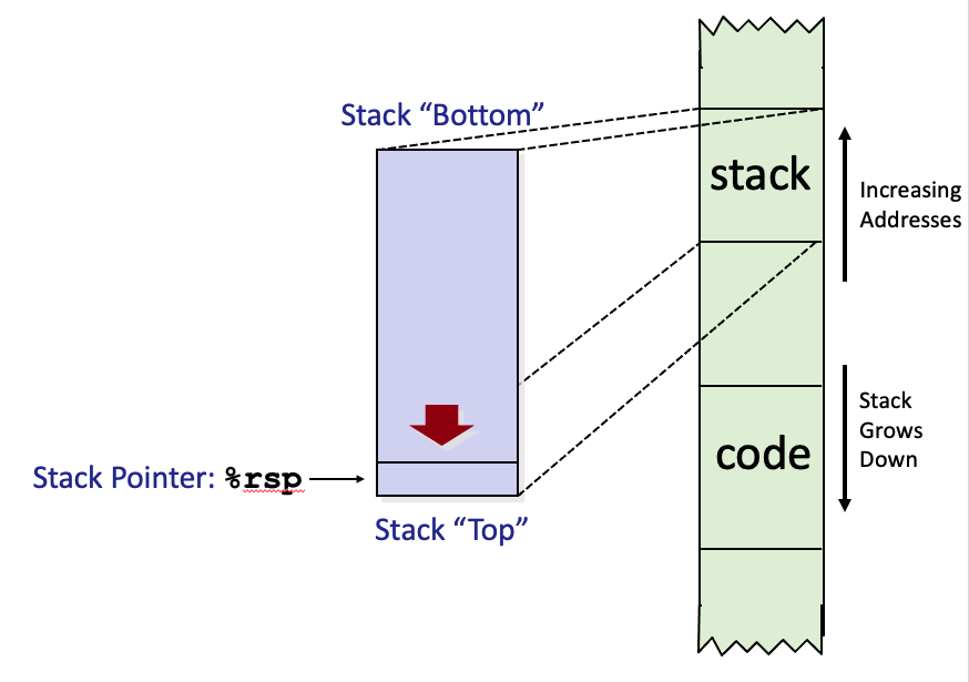
30. x86-64 stack

• Region of memory managed with stack discipline
  • Memory viewed as array of bytes.
  • Different regions have different purposes.
  • (Like ABI, a policy decision)
• Grows toward lower addresses
  • Register %rsp contains lowest stack address.
  • address of “top” element

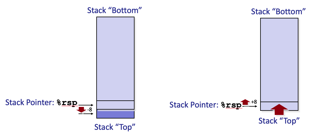
31. Stack push and pop

• pushq Src
  • Fetch operand at Src
  • Decrement %rsp by 8
  • Write operand at address given by %rsp
• popq Dest
  • Read value at address given by %rsp
  • Increment %rsp by 8
  • Store value at Dest (usually a register)

32. Hands on: function calls

• Create a file named mult.c in 04-machine with the following contents:

• Compile with -g and -Og flags and run gdb on the resulting executable.

$ gcc -g -Og -o mult mult.c
$ gdb mult

• Setup gdb with a breakpoint at main and start running.
• A new GDB command is s or step: executing the next instruction (machine or code instruction).
  • It will execute the highlighted (greened and arrowed) instruction in the code section.
• Be careful, Intel notation in the code segment of GDB
• Run s once to execute sub rsp,0x8

• Use n to execute the instruction: mov edi,0x8 and step over the next instruction, call 0x0400410 <malloc@plt>, which is a function call that we don’t want to step into this call.
• These are the instructions for the malloc call.

mov edi,0x8
call 0x0400410 <malloc@plt>

• Pay attention to the next three instructions after call 0x0400410 <malloc@plt.
  • Recall that the return value of malloc is placed into %rax.
• These instructions setup the parameters for the upcoming multstore(1,2,p) call.
  • mov rdx,rax.
  • mov esi,0x2
  • mov edi,0x1
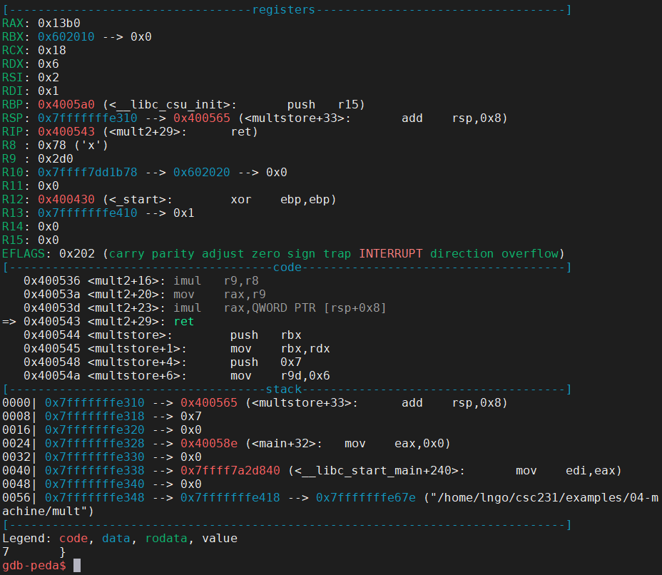
• Also, check the values of rax and p

gdb-peda$ p $rax
gdb-peda$ p p

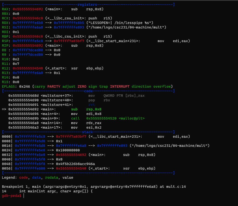
• This is the value of the memory block allocated via malloc to contain one long element.
• Run s to step into multstore(1,2,p)

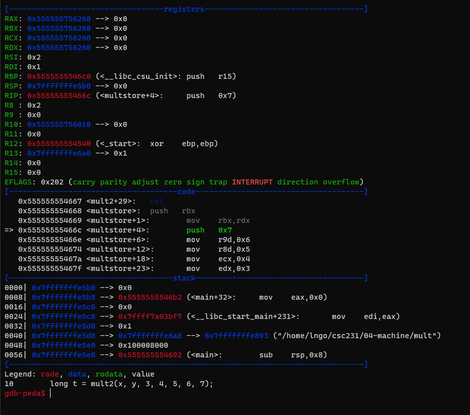
• Inside mulstore, we immediately prepare to launch mult2.
• Run s once. This will store the value in rdx into rbx. This is to save the value in rdx because we need to use it later. parameters for the mult2 call.
• Procedure Data Flow:
  • First six parameters will be placed into rdi, rsi, rdx, rcx, r8, r9.
  • The remaining parameters will be pushed on to the stack of the calling function ( in this case mulstore).
  • Note that rsp (stack pointer of multstore) is currently at 0x7ffffffe320.
• Run s to step into mult2.

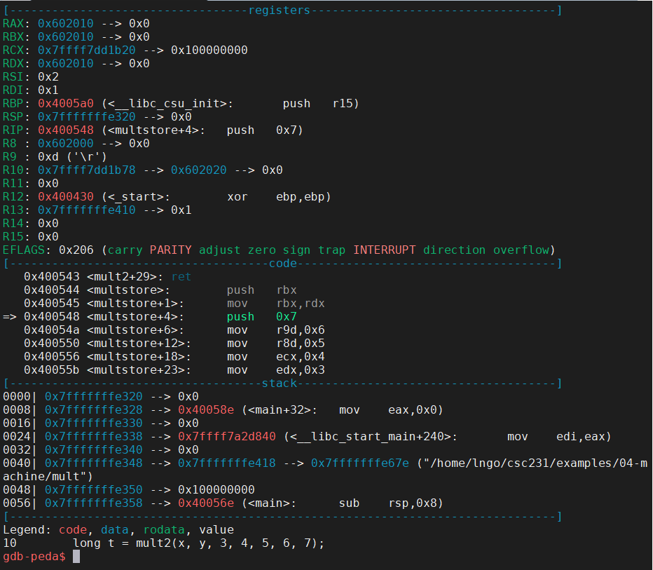
• The 7^th parameter of mult2 is pushed on to the stack frame of multstore and is stored at address 0x7ffffffe318.
• Function/procedure mult2 has no local variable, hence the stack frame is almost empty. The stack pointer, rsp, of mult2, is actually pointing toward the address of the 7^th parameter.
• Run s.
• The subsequence instructions (<mult2> through <mult2+23>) are for the multiplication.
• The final value will be stored in rax to be returned to multstore.
• Examine the two screenshots below to see how specific registers contain certain values?
  • rcx?
  • r8?
  • r9?
  • What is value of rax after <mult2+20>?
  • What is value of rax after <mult2+23>?

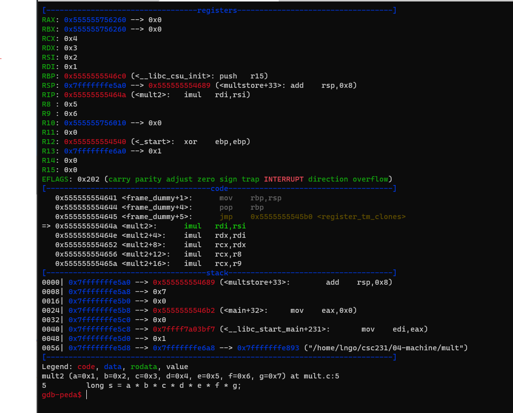
• Continue running s to finish the program.

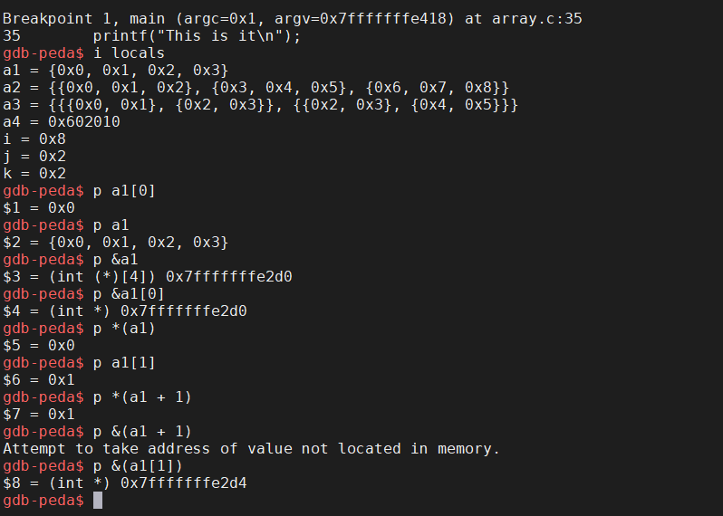
33. Hands on: array and multi-dimensional arrays

• Given array of data type T and length L: T A[L]
  • Contiguous allocated region of L * sizeof(T) bytes in memory.
  • Identifier A can be used as a pointer to array element 0.
• Create a file named array.c in 04-machine with the following contents:

• Run cat -n array.c and remember the line number of the printf statement.
• Compile with -g flag and run gdb on the resulting executable.

$ cat -n array.c
$ gcc -g -o array array.c
$ gdb array

• Setup gdb with a breakpoint at the line number for the printf statement and start running.
• Run i locals to view all local variables.
• Use p and variety of pointer/array syntax to view their values and addresses: *, [], &.

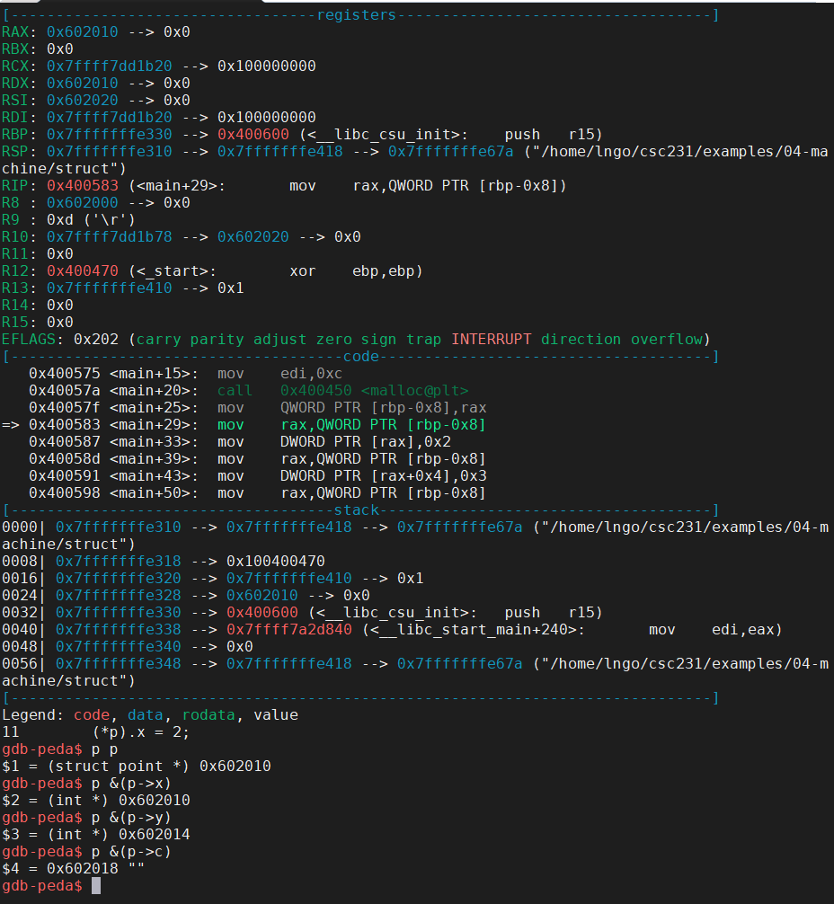
34. Hands on: struct

• Create a new data type (non-primitive) that groups objects of possibly different types into a single object.
  • Think classes in object-oriented programming minus the methods.
• Create a file named struct.c in 04-machine with the following contents:

• Compile with -g flag and run gdb on the resulting executable.

$ gcc -g -o struct struct.c
$ gdb struct

• Setup gdb with a breakpoint at main` and start running.
• Use n to walk through the program and answer the following questions:
  • How many bytes are there in the memory block allocated for variable p?
  • How are the addresses of x, y, and c relative to p?

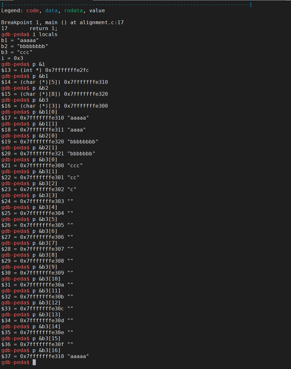
35. Data alignment

• Intel recommends data to be aligned to improve memory system performance.
  • K-alignment rule: Any primitive object of K bytes must have an address that is multiple of K: 1 for char, 2 for short, 4 for int and float, and 8 for long, double, and char *.
• Create a file named alignment.c in 04-machine with the following contents:

• Run cat -n alignment.c and remember the line number of the return statement.
• Compile with -g flag and run gdb on the resulting executable.

$ cat -n array.c
$ gcc -g -o array array.c
$ gdb array
gdb-peda$ b 17
gdb-peda$ run

• Run i locals to view all local variables.
• Use p and & to view addresses of the three char array variables and the i variable.
• Why does address displacement is not an exact match between the i variable and the next array variable versus between the array variables?

Key Points

• First key point. Brief Answer to questions. (FIXME)

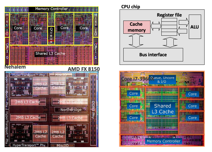
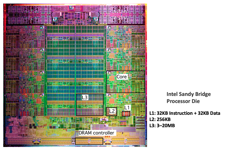
Memory hierarchy and cache memories

Overview

Teaching: 0 min
Exercises: 0 min

Questions

• What else is there besides RAM?

• How different levels of the memory hierarchy can affect performance?

Objectives

• Know the different levels of the memory hierarchy.

• Understand performance differences in accessing different memory levels.

1. Memory abstraction: writing and reading memory

• Write:
  • Transfer data from CPU to memory: movq 8(%rsp), %rax
  • Store operation
• Read:
  • Trasnfer data from memory to CPU: movq %rax, 8(%rbp)
  • Load operation
• Physical representation of this abstraction:

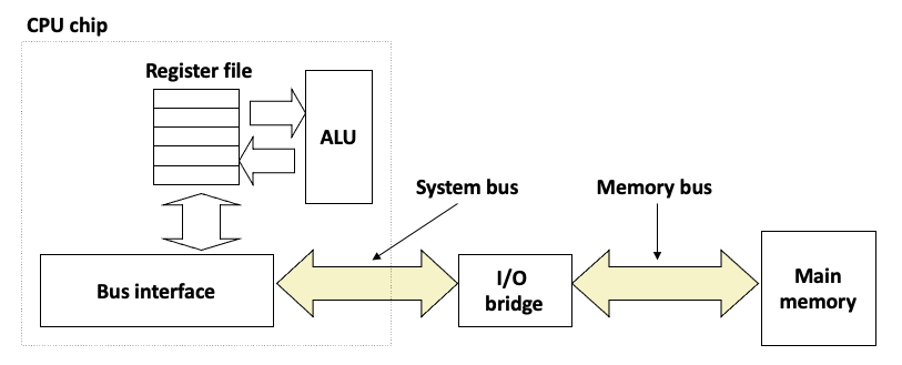
2. Random-Access Memory (RAM)

• Key features:
  • RAM is traditionally packaged as a chip, or embedded as part of processor chip
  • Basic storage unit is normally a cell (one bit per cell).
  • Multiple RAM chips form a memory.
• RAM comes in two varieties:
  • SRAM (Static RAM): transistors only
  • DRAM (Dynamic RAM): transistor and capacitor

  • Both are volatile: memory goes away without power.

    Transistor per bit	Access time	Need refresh	Needs EDC	Cost	Applications
    SRAM	6 or 8	1x	No	Maybe	100x	Cache memories
    DRAM	1	10x	Yes	Yes	1x	Main memories, frame buffers

EDC: Error Detection and Correction

• Trends:
  • SRAM scales with semiconductor technology
    • Reaching its limits
  • DRAM scaling limited by need for minimum capacitance
    • Aspect ratio limits how deep can make capacitor
    • Also reaching its limits

3. Enhanced DRAMs

• Operation of DRAM cell has not changed since its invention
  • Commercialized by Intel in 1970.
• DRAM cores with better interface logic and faster I/O :
  • Synchronous DRAM (SDRAM)
    • Uses a conventional clock signal instead of asynchronous control
  • Double data-rate synchronous DRAM (DDR SDRAM)
    • Double edge clocking sends two bits per cycle per pin
    • Different types distinguished by size of small prefetch buffer:
      • DDR (2 bits), DDR2 (4 bits), DDR3 (8 bits), DDR4 (16 bits)
    • By 2010, standard for most server and desktop systems
  • Intel Core i7 supports DDR3 and DDR4 SDRAM

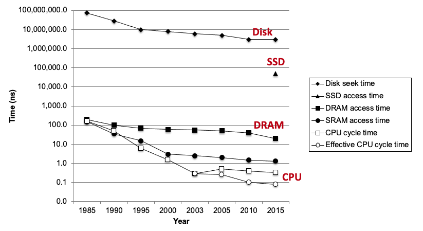
4. The CPU-Memory gap

• The key to bridging this gap is a fundamental property of computer programs known as locality:
  • Principle of Locality: Programs tend to use data and instructions with addresses near or equal to those they have used recently
  • Temporal locality: Recently referenced items are likely to be referenced again in the near future
  • Spatial locality: Items with nearby addresses tend to be referenced close together in time

sum = 0;
for (i = 0; i < n; i++)
  sum += a[i];
return sum;

• Data references
  • Reference array elements in succession (stride-1 reference pattern): spatial
  • Reference variable sum each iteration: temporal
• Instruction references
  • Reference instructions in sequence: spatial
  • Cycle through loop repeatedly: temporal

5. Qualitative estimates of locality

• Being able to look at code and get a qualitative sense of its locality is among the key skills for a professional programmer.

Exercise 1

Does this function have good locality with respect to array a?

int sum_array_rows(int a[M][N]) {
  int i, j, sum = 0;
  for (i = 0; i < M; i++)
    for (j = 0; j < N; j++)
      sum += a[i][j];
  return sum;
}

Hint: array layout is row-major order

Answer

Yes

Exercise 2

Does this function have good locality with respect to array a?

int sum_array_rows(int a[M][N]) {
  int i, j, sum = 0;
  for (j = 0; j < N; j++)
    for (i = 0; i < M; i++)
      sum += a[i][j];
  return sum;
}

Hint: array layout is row-major order

Answer

No

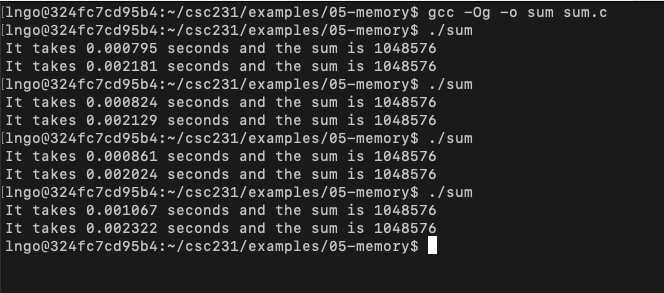
6. Hands on: performance measurement of locality

• In your home directory, create a directory called 05-memory and change into this directory.
• Create a file named sum.c with the following contents:

• Compile and run several times.
• Observe the performance difference.

$ gcc -Og -o sum sum.c
$ ./sum
$ ./sum
$ ./sum
$ ./sum

7. Memory hierarchies

• Some fundamental and enduring properties of hardware and software:
  • Fast storage technologies cost more per byte, have less capacity, and require more power (heat!).
  • The gap between CPU and main memory speed is widening.
  • Well-written programs tend to exhibit good locality.
• These fundamental properties complement each other beautifully.
• They suggest an approach for organizing memory and storage systems known as a memory hierarchy.

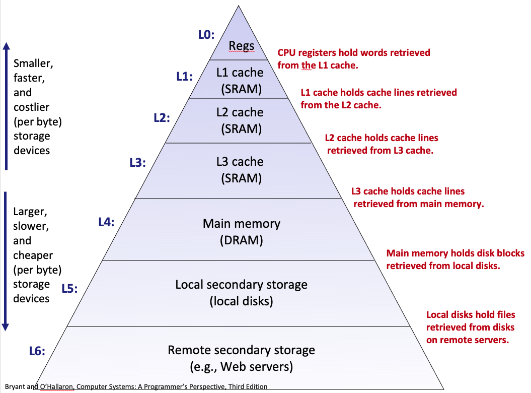
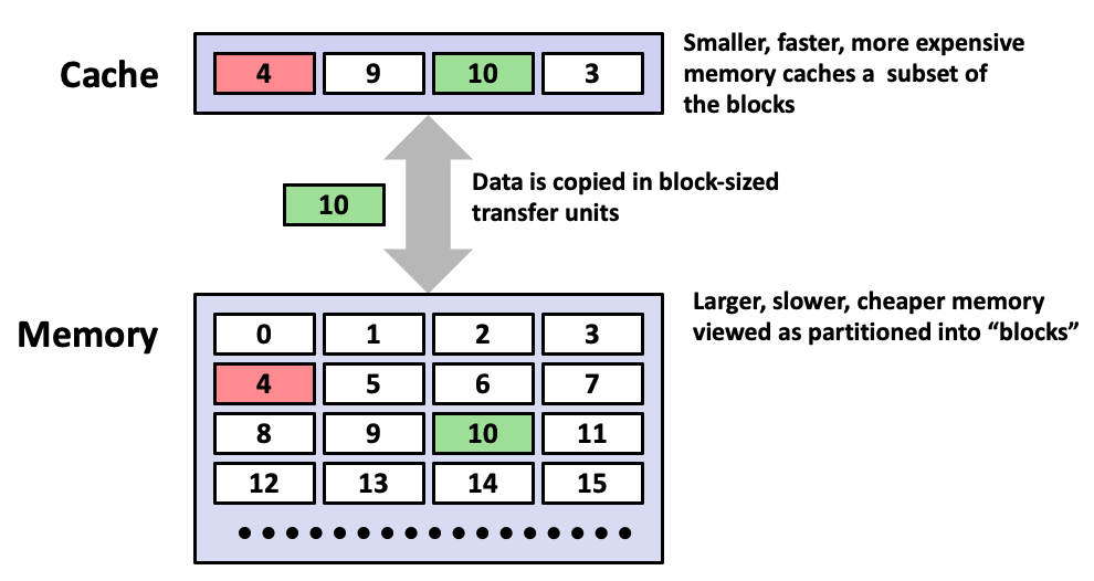
8. Caching

• Cache: A smaller, faster storage device that acts as a staging area for a subset of the data in a larger, slower device.
• Fundamental idea of a memory hierarchy:
  • For each k, the faster, smaller device at level k serves as a cache for the larger, slower device at level k+1.
• Why do memory hierarchies work?
  • Because of locality, programs tend to access the data at level k more often than they access the data at level k+1.
  • Thus, the storage at level k+1 can be slower, and thus larger and cheaper per bit.
• Big Idea (Ideal): The memory hierarchy creates a large poolof storage that costs as much as the cheap storage near the bottom, but that serves data to programs at the rate of the fast storage near the top.

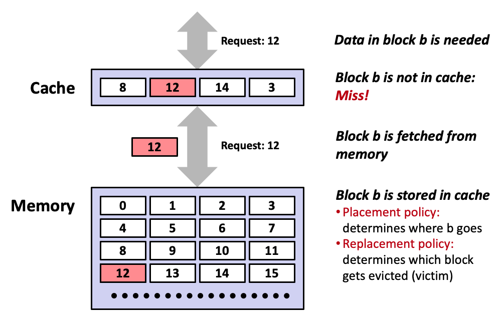
9. Caching: general concepts

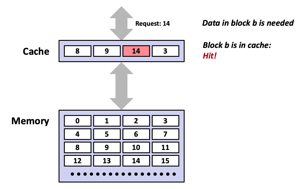
• Cold (compulsory) miss
  • Cold misses occur because the cache starts empty and this is the first reference to the block.
• Capacity miss
  • Occurs when the set of active cache blocks (working set) is larger than the cache.
• Conflict miss
  • Most caches limit blocks at level k+1 to a small subset (sometimes a singleton) of the block positions at level k.
    • E.g. Block i at level k+1 must be placed in block (i mod 4) at level k.
  • Conflict misses occur when the level k cache is large enough, but multiple data objects all map to the same level k block.
    • E.g. Referencing blocks 0, 8, 0, 8, 0, 8, … would miss every time.

Cache Type	What is cached	Where is it cached	Latency (cycles)	Managed By
Register	4-6 byte words	CPU core	0	Compiler
TLB	Address translations	On-chip TLB	0	Hardware MMU
L1 cache	64-byte blocks	On-chip L1	4	Hardware
L2 cache	64-byte blocks	On-chip L2	10	Hardware
Virtual memory	4-KB pages	Main memory	100	Hardware + OS
Buffer cache	Part of files	Main memory	100	OS
Disk cache	Disk sectors	Disk controller	100,000	Disk firmware
Network buffer cache	Part of files	Local disk	10,000,000	NFS client
Browser cache	Web pages	Local disk	10,000,000	Web browser
Web cache	Web pages	Remote server disks	1,000,000,000	Web proxy server

10. Cache memories

• Small, fast SRAM-based memories managed automatically in hardware.
• Hold frequently accessed blocks of main memory.
• CPU looks first for data in cache.

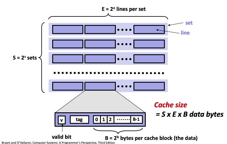
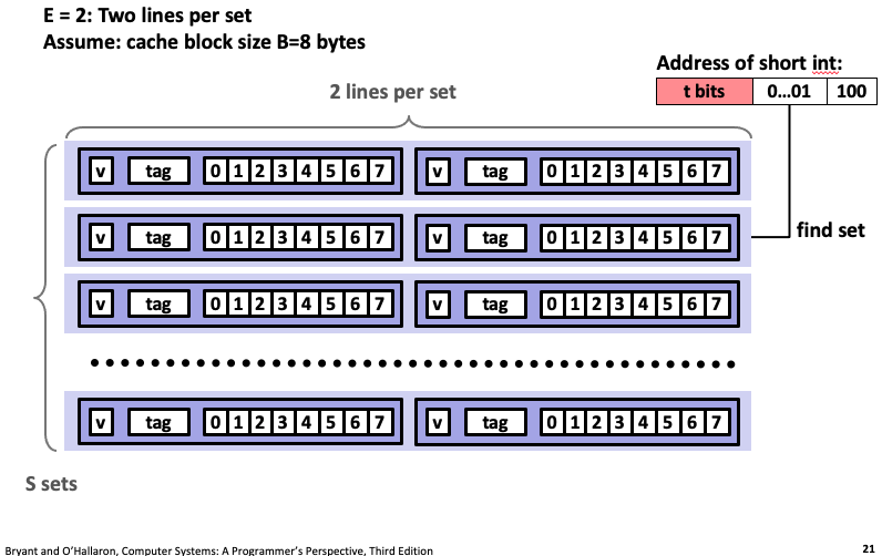
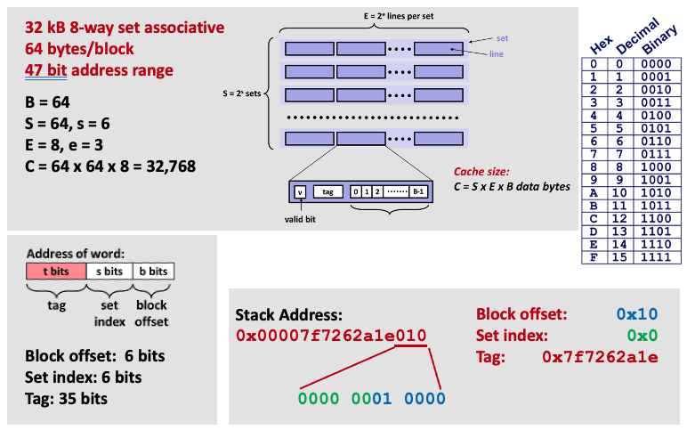
11. General cache organization

• Assume a computer system with m-bit addresses.
• Three values, S, E, and B represent the cache organization:
  • A cache for this system is organized as an array of S = 2^s cache sets.
  • Each set consists of E cache lines.
  • Each cache line has a data block of size B = 2^b bytes, a valid bit that indicates whether this line contains meaningful data, and a tag of size t bits: t = m - (b + s).
• Actual data address (m bits) are mapped to t, b, s to help determine whether the data is stored in cache.

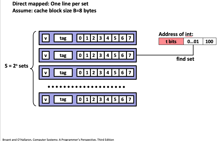
12. Example: direct mapped cache (E=1)

13. Example: two-way associative cache (E=2)

14. What about writes?

• Multiple copies of data exist:: L1, L2, L3, Main Memory, Disk
• What to do on a write-hit?
  • Write-through (write immediately to memory)
  • Write-back (defer write to memory until replacement of line)
    • Each cache line needs a dirty bit (set if data differs from memory)
• What to do on a write-miss?
  • Write-allocate (load into cache, update line in cache): Good if more writes to the location will follow
  • No-write-allocate (writes straight to memory, does not load into cache)
• Typical
  • Write-through + No-write-allocate
  • Write-back + Write-allocate

15. Example: Core i7 L1 Data Cache

16. Cache performance metrics

• Miss Rate
  • Fraction of memory references not found in cache (misses / accesses) = 1 – hit rate
  • Typical numbers (in percentages):
    • 3-10% for L1
    • can be quite small (e.g., < 1%) for L2, depending on size, etc.
• Hit Time
  • Time to deliver a line in the cache to the processor
    • includes time to determine whether the line is in the cache
  • Typical numbers:
    • 4 clock cycle for L1
    • 10 clock cycles for L2
• Miss Penalty
  • Additional time required because of a miss
    • typically 50-200 cycles for main memory (Trend: increasing!)

17. What those numbers mean?

• Huge difference between a hit and a miss
  • Could be 100x, if just L1 and main memory
• Would you believe 99% hits is twice as good as 97%?
  • Consider this simplified example:
    • cache hit time of 1 cycle
    • miss penalty of 100 cycles
  • Average access time:
    • 97% hits: 1 cycle + 0.03 x 100 cycles = 4 cycles
    • 99% hits: 1 cycle + 0.01 x 100 cycles = 2 cycles
• This is why miss rate is used instead of hit rate.

18. Write cache friendly code

• Make the common case go fast
  • Focus on the inner loops of the core functions
• Minimize the misses in the inner loops
  • Repeated references to variables are good (temporal locality)
  • Stride-1 reference patterns are good (spatial locality)
• Key idea: our qualitative notion of locality is quantified through our understanding of cache memories.

19. Matrix multiplication example

• Multiply N x N matrices
• Matrix elements are doubles (8 bytes)
• O(N³) total operations
• N reads per source element
• N values summed per destination but may be able to hold in register

20. Miss rate analysis for matrix multiply

• Assume:
  • Block size = 32B (big enough for four doubles)
  • Matrix dimension (N) is very large: Approximate 1/N as 0.0
  • Cache is not even big enough to hold multiple rows
• Analysis Method:
  • Look at access pattern of inner loop

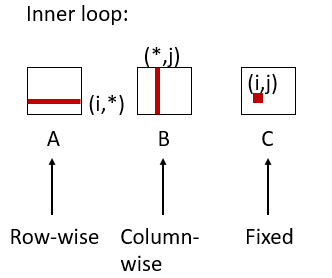
/* ijk */
for (i=0; i<n; i++)  {
  for (j=0; j<n; j++) {
    sum = 0.0;
    for (k=0; k<n; k++) 
      sum += a[i][k] * b[k][j];
    c[i][j] = sum;
  }
} 

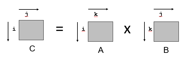
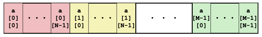
21. Layout of C arrays in memory

• C arrays allocated in row-major order
  • each row in contiguous memory locations
• Stepping through columns in one row:
  • for (i = 0; i < N; i++)
    sum += a[0][i];
  • accesses successive elements
  • if block size (B) > sizeof(a^ij) bytes, exploit spatial locality
    • miss rate = sizeof(a^ij) / B
• Stepping through rows in one column:
  • for (i = 0; i < n; i++)
    sum += a[i][0];
  • accesses distant elements
  • no spatial locality!
  • miss rate = 1 (i.e. 100%)

22. Matrix multiplication

• C arrays allocated in row-major order

/* ijk */
for (i=0; i<n; i++)  {
  for (j=0; j<n; j++) {
    sum = 0.0;
    for (k=0; k<n; k++) 
      sum += a[i][k] * b[k][j];
    c[i][j] = sum;
  }
} 

• Miss rate for inner loop iterations:
• Block size = 32 bytes (4 doubles)
  • A = 8 / 32 = 0.25
  • B = 1
  • C = 0
  • Average miss per iteration = 1.25

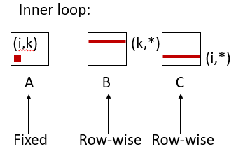
/* kij */
for (k=0; k<n; k++)  {
  for (i=0; i<n; i++) {
    r = a[i][k];
    for (j=0; j<n; j++) 
      c[i][j] += r * b[k][j];
  }
} 

• Miss rate for inner loop iterations:
• Block size = 32 bytes (4 doubles)
  • A = 0
  • B = 8 / 32 = 0.25
  • C = 8 / 32 = 0.25
  • Average miss per iteration = 0.5

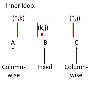
/* jki */
for (j=0; j<n; j++)  {
  for (k=0; k<n; k++) {
    r = b[k][j];
    for (i=0; i<n; i++) 
      c[i][j] += a[i][k] * r;
  }
} 

• Miss rate for inner loop iterations:
• Block size = 32 bytes (4 doubles)
  • A = 1
  • B = 0
  • C = 1
  • Average miss per iteration = 2

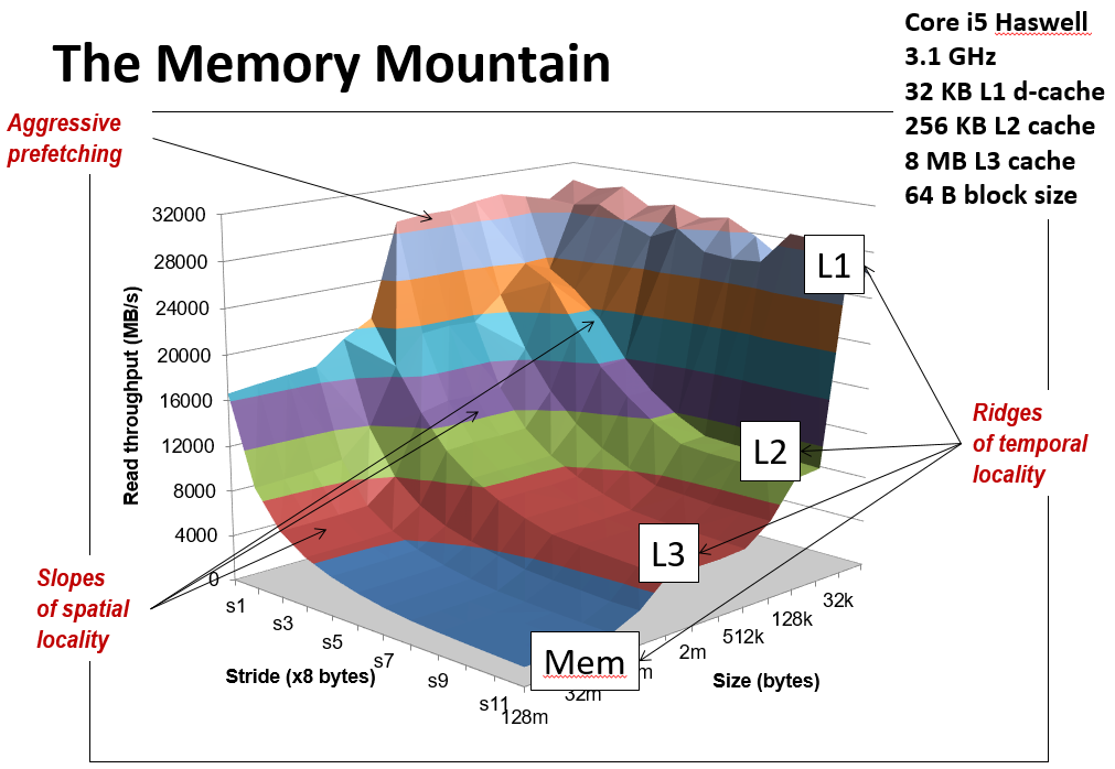
23. The memory mountain

• This is the cover of the book.
• Y-axis: Read throughput (read bandwidth)
  • Number of bytes read from memory per second (MB/s)
• Memory mountain: Measured read throughput as a function of spatial and temporal locality.
• Compact way to characterize memory system performance.

Key Points

• First key point. Brief Answer to questions. (FIXME)

C programming debugging and optimization

Overview

Teaching: 0 min
Exercises: 0 min

Questions

• How can programs run faster?

Objectives

• First learning objective. (FIXME)

1. Defects and Infections

• A systematic approach to debugging.
  • The programmer creates a defect
  • The defect causes an infection
  • The infection propagates
  • The infection causes a failure
• Not every defect causes a failure!
• Testing can only show the presence of errors - not their absence.
  • In other words, if you pass every tests, it means that your program has yet to fail. It does not mean that your program is correct.

2. Explicit debugging

• Stating the problem
  • Describe the problem aloud or in writing
  • A.k.a. Rubber duck or teddy bear method
• Often a comprehensive problem description is sufficient to solve the failure

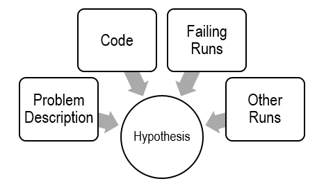
3. Scientific debugging

• Before debugging, you need to construct a hypothesis as to the defect.
  • Propose a possible defect and why it explains the failure conditions
• Ockham’s Razor: given several hypotheses, pick the simplest/closest to current work

• Make predictions based on your hypothesis
  • What do you expect to happen under new conditions
  • What data could confirm or refute your hypothesis
• How can I collect that data?
  • What experiments?
  • What collection mechanism?
• Does the data refute the hypothesis?
  • Refine the hypothesis based on the new inputs

4. Hands on: bad Fibonacci

• Specification defined the first Fibonacci number as 1.
• Compile and run the following bad_fib.c program:
• fib(1) returns an incorrect result. Why?

$ gcc -o bad_fib bad_fib.c
$ ./bad_fib

• Constructing a hypothesis:
  • while (n > 1): did we mess up the loop in fib?
  • int f: did we forget to initialize f?
• Propose a new condition or conditions
  • What will logically happen if your hypothesis is correct?
  • What data can be
  • fib(1) failed // Hypothesis
    • Loop check is incorrect: Change to n >= 1 and run again.
    • f is uninitialized: Change to int f = 1;
• Experiment
  • Only change one condition at a time.
  • fib(1) failed // Hypothesis
    • Change to n >= 1: ???
    • Change to int f = 1: Works. Sometimes a prediction can be a fix.

5. Hands on: brute force approach

• Strict compilation flags: -Wall, -Werror.
• Include optimization flags (capital letter o): -O3 or -O0.

$ gcc -Wall -Werror -O3 -o bad_fib bad_fib.c

• Use valgrind, memory analyzer.

$ sudo apt-get install -y valgrind
$ gcc -Wall -Werror -o bad_fib bad_fib.c
$ valgrind ./bad_fib

6. Observation

• What is the observed result?
  • Factual observation, such as Calling fib(1) will return 1.
  • The conclusion will interpret the observation(s)
• Don’t interfere.
  • Sometimes printf() can interfere
  • Like quantum physics, sometimes observations are part of the experiment
• Proceed systematically.
  • Update the conditions incrementally so each observation relates to a specific change
• Do NOT ever proceed past first bug.

7. Learn

• Common failures and insights
  • Why did the code fail?
  • What are my common defects?
• Assertions and invariants
  • Add checks for expected behavior
  • Extend checks to detect the fixed failure
• Testing
  • Every successful set of conditions is added to the test suite

8. Quick and dirty

• Not every problem needs scientific debugging
• Set a time limit: (for example)
  • 0 minutes – -Wall, valgrind
  • 1 – 10 minutes – Informal Debugging
  • 10 – 60 minutes – Scientific Debugging
  • 60 minutes – Take a break / Ask for help

8. Code optimization: Rear Admiral Grace Hopper

• Invented first compiler in 1951 (technically it was a linker)
• Coined compiler (and bug)
• Compiled for Harvard Mark I
• Eventually led to COBOL (which ran the world for years)
• “I decided data processors ought to be able to write their programs in English, and the computers would translate them into machine code”.

9. Code optimization: John Backus

• Led team at IBM invented the first commercially available compiler in 1957
• Compiled FORTRAN code for the IBM 704 computer
• FORTRAN still in use today for high performance code
• “Much of my work has come from being lazy. I didn’t like writing programs, and so, when I was working on the IBM 701, I started work on a programming system to make it easier to write programs”.

10. Code optimization: Fran Allen

• Pioneer of many optimizing compilation techniques
• Wrote a paper simply called Program Optimization in 1966
• “This paper introduced the use of graph-theoretic structures to encode program content in order to automatically and efficiently derive relationships and identify opportunities for optimization”.
• First woman to win the ACM Turing Award (the Nobel Prize of Computer Science).

11. Performance realities

• There’s more to performance than asymptotic complexity.
• Constant factors matter too!
  • Easily see 10:1 performance range depending on how code is written
  • Must optimize at multiple levels: algorithm, data representations, procedures, and loops
• Must understand system to optimize performance
  • How programs are compiled and executed
  • How modern processors + memory systems operate
  • How to measure program performance and identify bottlenecks
  • How to improve performance without destroying code modularity and generality.

12. Leveraging cache blocks

• Check the size of cache blocks

$ getconf -a | grep CACHE

• We focus on cache blocks for optimization:
  • If calculations can be performed using smaller matrices of A, B, and C (blocks) that all fit in cache, we can further minimize the amount of cache misses per calculation.

• 3 blocks are needed (for A, B, and C).
• Each block has dimension B, so the total block size is B²
• Therefore: 3B² < cache_size
• Based on the information above: B = 8 (so that 8 * 8 = 64 fits in cache line).
• 3 * 8 * 8 < 32768.

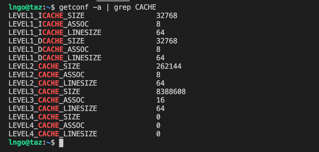
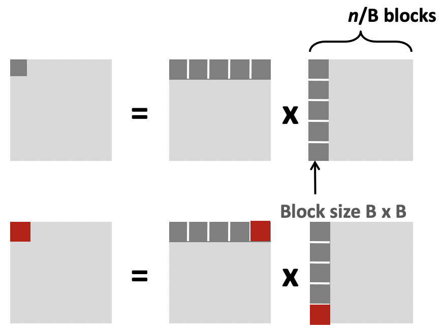
13. Hands-on: matrix multiplications

• Check the size of cache blocks

$ getconf -a | grep CACHE

• Create the following two files: matrix_mult.c and block_matrix_mult.c inside a directory called 06-optimization.

• Compile and run the two files:

$ gcc -o mm matrix_mult.c
$ ./mm 512
$ ./mm 1024
$ ./mm 2048
$ gcc -o bmm block_matrix_mult.c
$ ./bmm 512
$ ./bmm 1024
$ ./bmm 2048

• Repeat the process with optimized compilation flag O3:

$ gcc -O3 -o mm matrix_mult.c
$ ./mm 512
$ ./mm 1024
$ ./mm 2048
$ gcc -O3 -o bmm block_matrix_mult.c
$ ./bmm 512
$ ./bmm 1024
$ ./bmm 2048

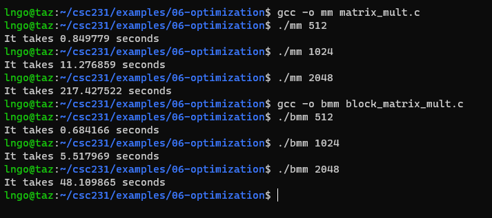
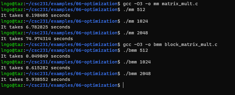
14. General optimization: you or your compiler should do it.

• Reduce code motion: reduce frequency with which computation performed
  • Need to produce same results
  • Move code out of loop.

• Reduction in strength: replace costly operation with simpler ones (multiply to addition).
  • Recognize sequence of products.

• Create the following file to automate the installations.

$ chmod 755 eval.sh
$ ./eval.sh block_matrix_mult
$ ./eval.sh block_matrix_mult_2
$ ./eval.sh block_matrix_mult_3

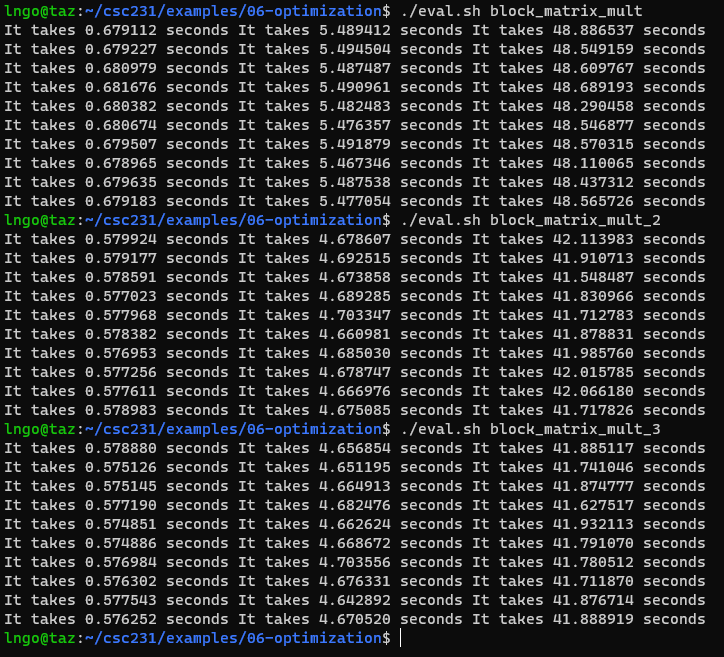
15. General optimization: when your compiler can’t.

• Operate under fundamental constraint
• Must not cause any change in program behavior
• Often prevents optimizations that affect only “edge case” behavior
• Behavior obvious to the programmer is not obvious to compiler
  • e.g., Data range may be more limited than types suggest (short vs. int)
• Most analysis is only within a procedure
  • Whole-program analysis is usually too expensive
  • Sometimes compiler does interprocedural analysis within a file (new GCC)
• Most analysis is based only on static information
  • Compiler has difficulty anticipating run-time inputs
• When in doubt, the compiler must be conservative

Key Points

• First key point. Brief Answer to questions. (FIXME)

Network programming

Overview

Teaching: 0 min
Exercises: 0 min

Questions

• Introduction to network programming

Objectives

• First learning objective. (FIXME)

1. In the beginning

• 1966: Advanced Research Projects Agency Network (ARPANET) - DOD
• 1969: Four sites:
  • SRI: Stanford Research Institutte
  • Utah: University of Utah
  • UCLA
  • UCSB

• 1977: East and West
  • MITRE Corporation: managed federally funded research and development centers (FFRDC) for a number of U.S. agencies (DOD, FAA, IRS, DVA, DHS, AO, CMMS, NIST)
  • BNN: now a subsidiary of Raytheon
  • Burroughs: now part of Unisys

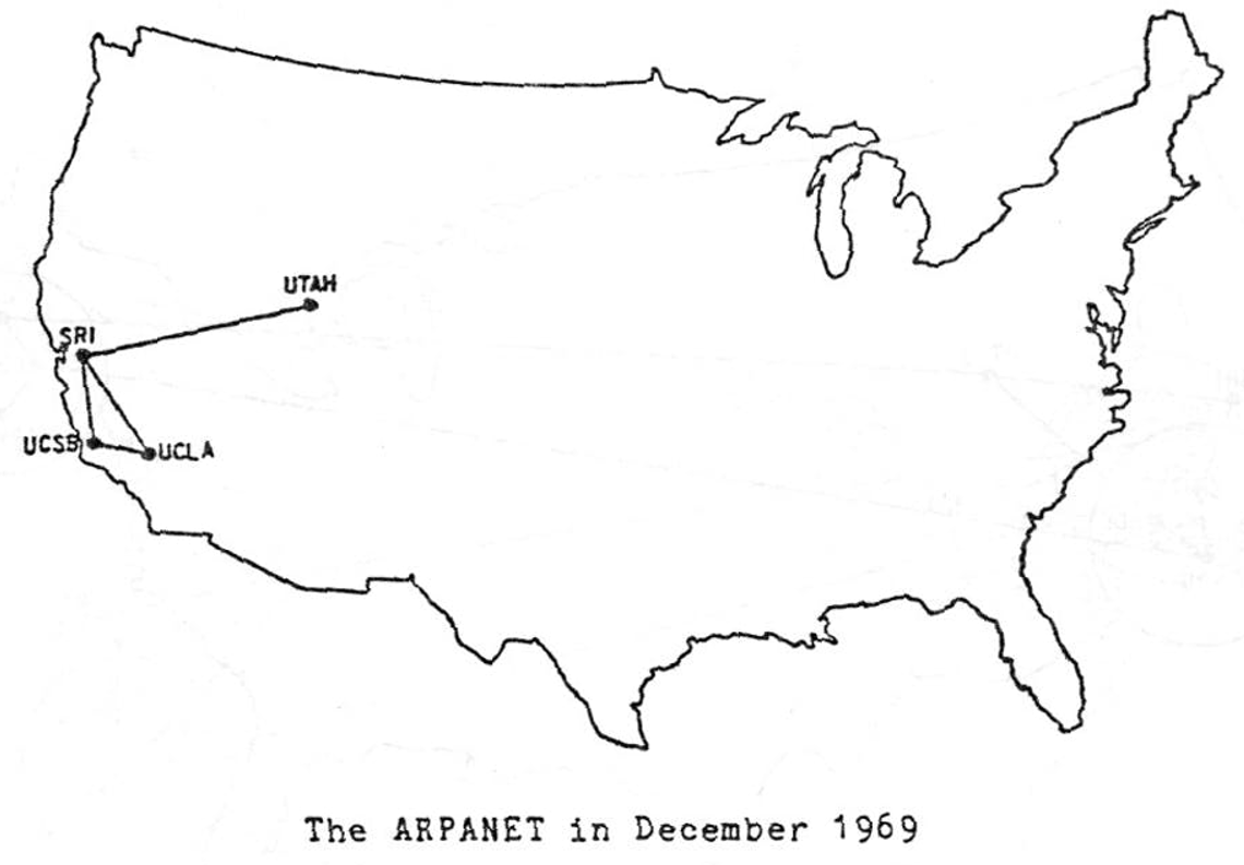
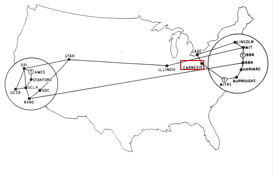
2. Now

• 2012: the Carna Botnet was unleashed.
  • An ethical hacking experiment in 2012 that used Nmap Scripting Engine (NSE) to scan for random devices with default telnet login username and password.
  • Over 100,000 devices had these features and could easily be accessed.
  • A spider-like crawling approach was used to have the vulnerable devices to scan for other vulnerable devices.
  • In the end, a total of 420,000 devices were assisting the internet search, and of the 4.3 billion IP addresses possible, the Carna Botnet found 1.3 billion.
  • What came from the Carna Botnet was a massive census of the internet in 2012.

3. A client-server transaction

• Most network applications are based on the client-server model:
  • A server process and one or more client processes
  • Server manages some resource
  • Server provides service by manipulating resource for clients
  • Server activated by request from client (vending machine analogy)
• Clients and servers are processes running on hosts (can be the same or different hosts).

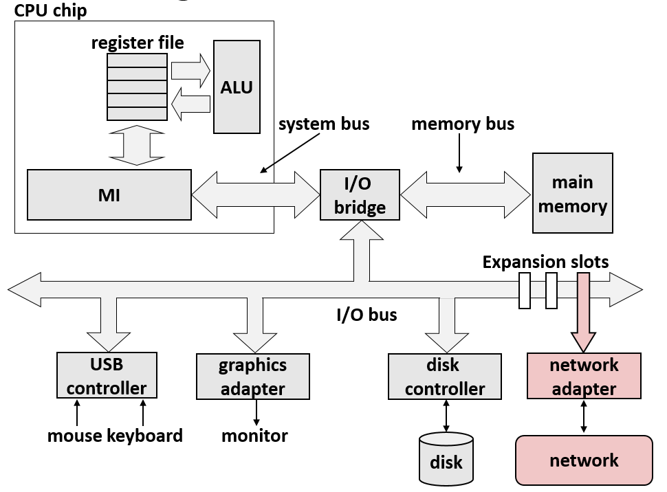
4. Computer networks

• A network is a hierarchical system of boxes and wires organized by geographical proximity
  • BAN (Body Area Network) spans devices carried / worn on body
  • SAN* (System Area Network) spans cluster or machine room
  • LAN (Local Area Network) spans a building or campus
  • WAN (Wide Area Network) spans country or world
• An internetwork (internet) is an interconnected set of networks

5. From the ground up

• Lowest level: Ethernet segments
  • consists of a collection of hosts connected by wires (twisted pairs) to a hub (replaced by switches and routers today).
  • Spans room or floor in a building
  • Each Ethernet adapter has a unique 48-bit address called MAC address: 00:16:ea:e3:54:e6
  • Hosts send bits to any other host in chunks called frames
  • Hub copies each bit from each port to every other port
    • Every host sees every bit
• Next level: bridged Ethernet segments.
  • Spans building or campus
  • Bridges cleverly learn which hosts are reachable from which ports and then selectively copy frames from port to port.
• Next level: Internet
  • Multiple incompatible LANs can be physically connected by specialized computers called routers.
  • The connected networks are called an internet (lower case)

6. Logical structure of an internet

• Ad hoc interconnection of networks
• No particular topology
• Vastly different router & link capacities
• Send packets from source to destination by hopping through networks
  • Router forms bridge from one network to another
  • Different packets may take different routes

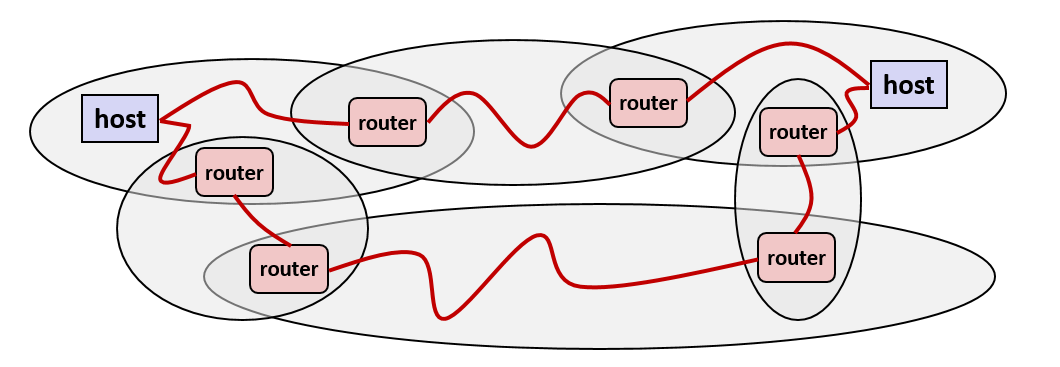
7. The notion of an internet protocol

• How is it possible to send bits across incompatible LANs and WANs?
• Solution: protocol software running on each host and router
  • Protocol is a set of rules that governs how hosts and routers should cooperate when they transfer data from network to network.
  • Smooths out the differences between the different networks

8. What does an internet protocol do?

• Provides a naming scheme
  • An internet protocol defines a uniform format for host addresses.
  • Each host (and router) is assigned at least one of these internet addresses that uniquely identifies it.
• Provides a delivery mechanism
  • An internet protocol defines a standard transfer unit (packet)
  • Packet consists of header and payload:
    • Header: contains info such as packet size, source and destination addresses
    • Payload: contains data bits sent from source host

9. Transferring internet data via encapsulation

• Ad hoc interconnection of networks
• No particular topology
• Vastly different router & link capacities
• Send packets from source to destination by hopping through networks
  • Router forms bridge from one network to another
  • Different packets may take different routes

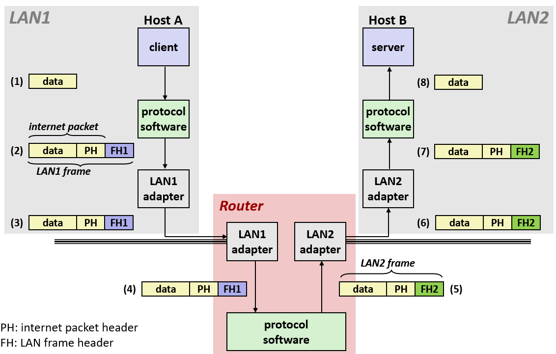
10. A trip down memory lane

11. Other issues

• We are glossing over a number of important questions:
  • What if different networks have different maximum frame sizes? (segmentation)
  • How do routers know where to forward frames?
  • How are routers informed when the network topology changes?
  • What if packets get lost?
• These (and other) questions are addressed by the area of systems known as computer networking

12. Global IP Internet (upper case)

• Most famous example of an internet
• Based on the TCP/IP protocol family
  • IP (Internet Protocol)
    • Provides basic naming scheme and unreliable delivery capability of packets (datagrams) from host-to-host
  • UDP (Unreliable Datagram Protocol)
    • Uses IP to provide unreliable datagram delivery from process-to-process.
  • TCP (Transmission Control Protocol)
    • Uses IP to provide reliable byte streams from process-to-process over connections.
• Accessed via a mix of Unix file I/O and functions from the sockets interface.

13. Hardware and software organization of an Internet Application

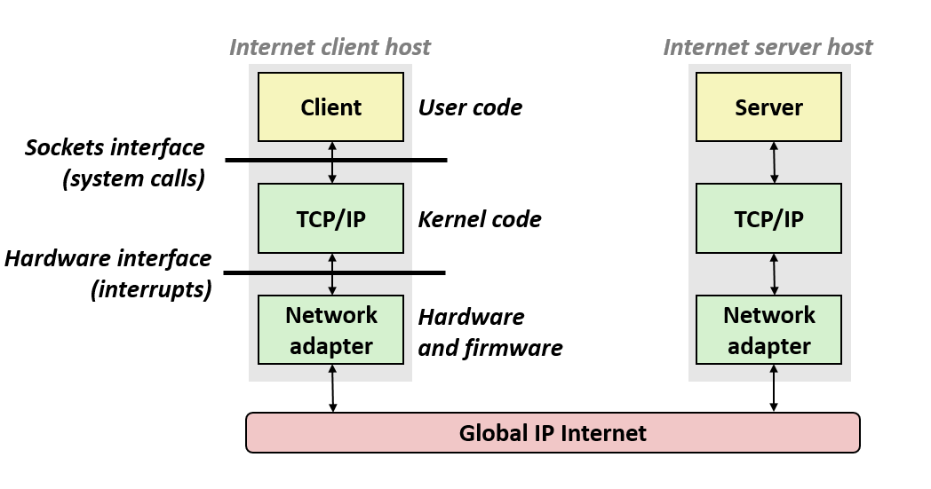
14. A programmer’s view of the Internet

• Hosts are mapped to a set of 32-bit IP addresses (lookout for IPv6 in the future)
  • 128.2.203.179
  • 127.0.0.1 (always localhost)
• The set of IP addresses is mapped to a set of identifiers called Internet domain names: 144.26.2.9 is mapped to www.wcupa.edu
• A process on one Internet host can communicate with a process on another Internet host over a connection.

15. IP addresses

• 32-bit IP addresses are stored in an IP address struct.
  • IP addresses are always stored in memory in network byte order (big-endian byte order)
  • True in general for any integer transferred in a packet header from one machine to another.
    • E.g., the port number used to identify an Internet connection

/* Internet address structure */
struct in_addr {
  uint32_t s_addr; /* network byte order (big-endian) */
};

• Dotted decimal notation
  • By convention, each byte in a 32-bit IP address is represented by its decimal value and separated by a period.
  • IP address: 0x8002C2F2 = 128.2.194.242
• Use getaddrinfo and getnameinfo functions (described later) to convert between IP addresses and dotted decimal format.
• Domain Naming System (DNS)
  • The Internet maintains a mapping between IP addresses and domain names in a huge worldwide distributed database called DNS.
  • Conceptually, programmers can view the DNS database as a collection of millions of host entries.
    • Each host entry defines the mapping between a set of domain names and IP addresses.
    • In a mathematical sense, a host entry is an equivalence class of domain names and IP addresses.

$ nslookup localhost
$ hostname -f
$ nslookup www.facebook.com
$ nslookup www.twitter.com

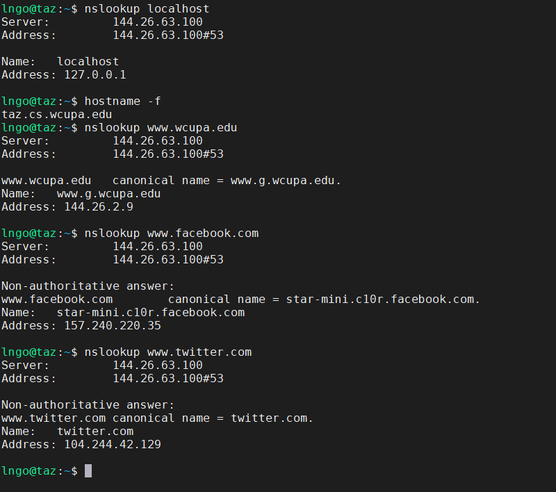
16. Internet connections

• Clients and servers communicate by sending streams of bytes over connections. Each connection is:
  • Point-to-point: connects a pair of processes.
  • Full-duplex: data can flow in both directions at the same time,
  • Reliable: stream of bytes sent by the source is eventually received by the destination in the same order it was sent.
• A socket is an endpoint of a connection
  • Socket address is an IPaddress:port pair
• A port is a 16-bit integer that identifies a process:
  • Ephemeral port: Assigned automatically by client kernel when client makes a connection request.
  • Well-known port: Associated with some service provided by a server (e.g., port 80 is associated with Web servers)

17. Well known service names and ports

• Popular services have permanently assigned well-known ports and corresponding well-known service names:
  • echo servers: echo 7
  • ftp servers: ftp 21
  • ssh servers: ssh 22
  • email servers: smtp 25
  • Web servers: http 80
• Mappings between well-known ports and service names is contained in the file /etc/services on each Linux machine.

18. Socket interface

• Set of system-level functions used in conjunction with Unix I/O to build network applications.
• Created in the early 80’s as part of the original Berkeley distribution of Unix that contained an early version of the Internet protocols.
• Available on all modern systems: Unix variants, Windows, OS X, IOS, Android, ARM
• What is a socket?
  • To the kernel, a socket is an endpoint of communication
  • To an application, a socket is a file descriptor that lets the application read/write from/to the network.
  • Remember: All Unix I/O devices, including networks, are modeled as files.
• Clients and servers communicate with each other by reading from and writing to socket descriptors.
• The main distinction between regular file I/O and socket I/O is how the application opens the socket descriptors.

19. Hands on: client/server network programming

• Create a directory called 07-networks.
• Create the following files server.c and client.c.

• Compile the two programs.
• Open a dual panel tmux and run server and client on each panel.
• Type strings into client and observe how it shows up on server.
• Type a corresponding string on server and observe how it shows on client.
• Type exit on each side to stop client and server.

$ gcc -o server server.c
$ gcc -o client client.c

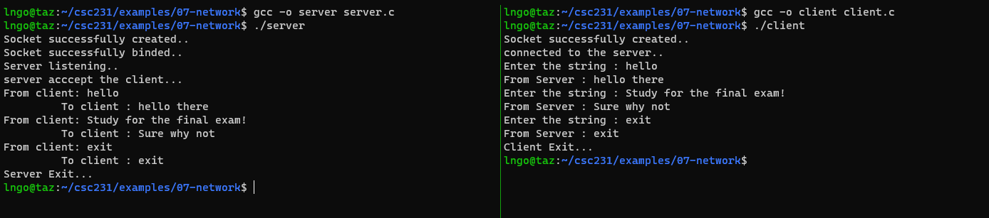
Key Points

• First key point. Brief Answer to questions. (FIXME)