Introduction to Operating Systems

Overview

Teaching: 0 min
Exercises: 0 min

Questions

What happens when a program run?

Objectives

Know the mechanisms that operating systems utilize to interface between users and hardware: virtualization and resource management

1. What happens when a computer program run?

The process

fetches an instruction from memory,

decodes the instruction, and

executes the instruction. This is the fundamental Von Neumann model of computing.

2. Why do we need OS?

What a programmer see is all code, lines of codes.

Underneath, there is a complex ecosystem of hardware components.

How do we hide this complexity away from the programmers?

3. How do the OS help (1)?

This is possible due to virtualization.

Virtualization: presents general, powerful, and easy-to-use virtual forms of physical computing resources to users (programmers).

The linkage between virtual interfaces and physical components are enabled through the OS’ system calls (or standard library).

4. How do the OS help (2)?

Each physical component in a computing system is considered a resource.

The OS manages these resources so that multiple programs can access these resources (through the corresponding virtual interface) at the same time.

This is called concurrency.

5. Hands-on: Getting started

Open a terminal (Windows Terminal or Mac Terminal).

Run the command to launch the image container for your platform:

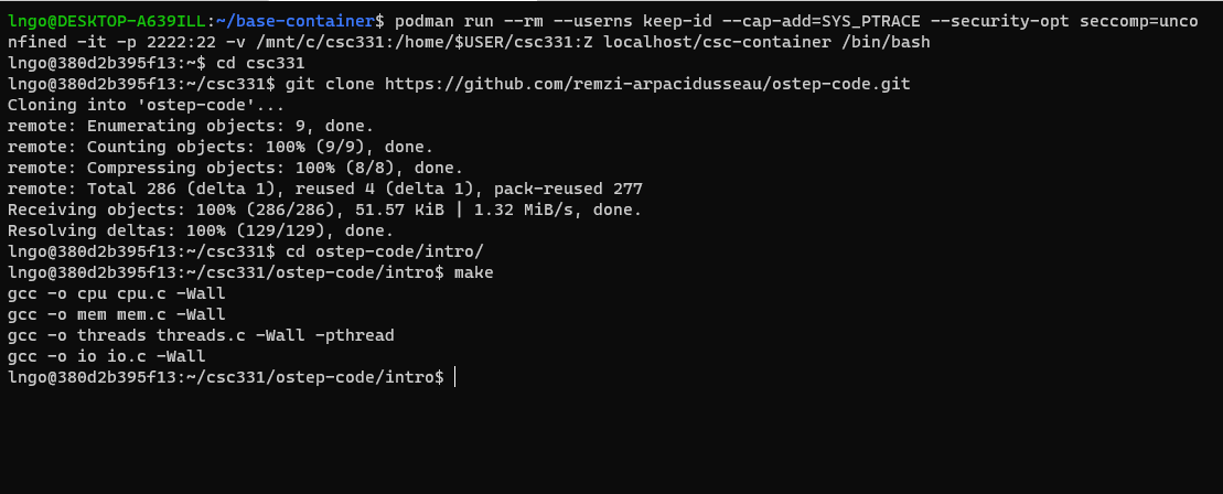
Windows:
$ podman run --rm --userns keep-id --cap-add=SYS_PTRACE --security-opt seccomp=unconfined -it -v /mnt/c/csc331:/home/$USER/csc331:Z localhost/csc-container /bin/bash
Mac:
$ docker run --rm --userns=host --cap-add=SYS_PTRACE --security-opt seccomp=unconfined -it -v /Users/$USER/csc331:/home/$USER/csc331:Z csc-container /bin/bash
Navigate to /home/$USER/csc331

Clone the scripts Dr. Arpaci-Dusseau’s Git repo.

Change to directory ostep-code/intro, then run make to build the programs.
$ git clone https://github.com/remzi-arpacidusseau/ostep-code.git
$ cd ostep-code/intro
$ make

6. Hands-on: CPU Virtualization

Our workspace is limited within the scope of a single terminal (a single shell) to interact with the operating system.

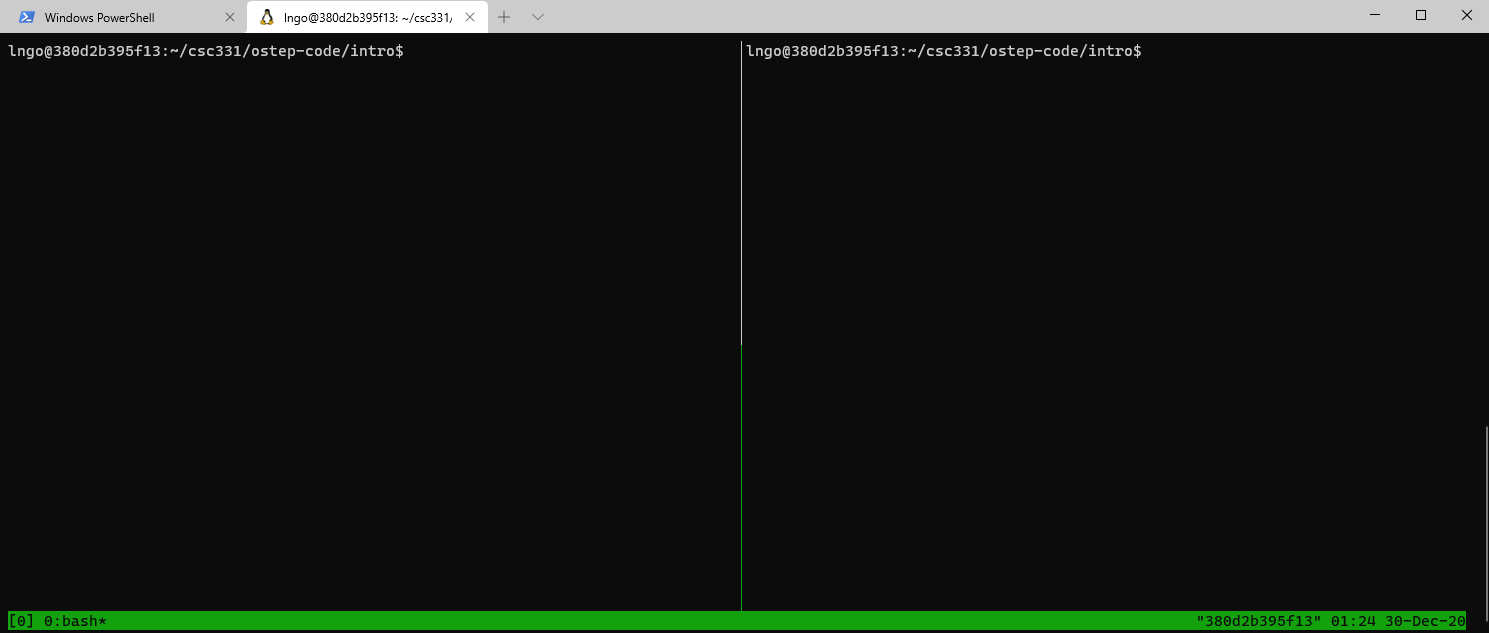
tmux: terminal multiplexer.

tmux allows user to open multiple terminals and organize split-views (panes) within these terminals within a single original terminal.

We can run/keep track off multiple programs within a single terminal.
$ cd ~/csc331/ostep-code/intro
$ tmux
Splits the tmux terminal into vertical panes: first press the keys Ctrl-b then lift your fingers and press the keys Shift-5 (technical documents > often write this as Ctrl-b and %).

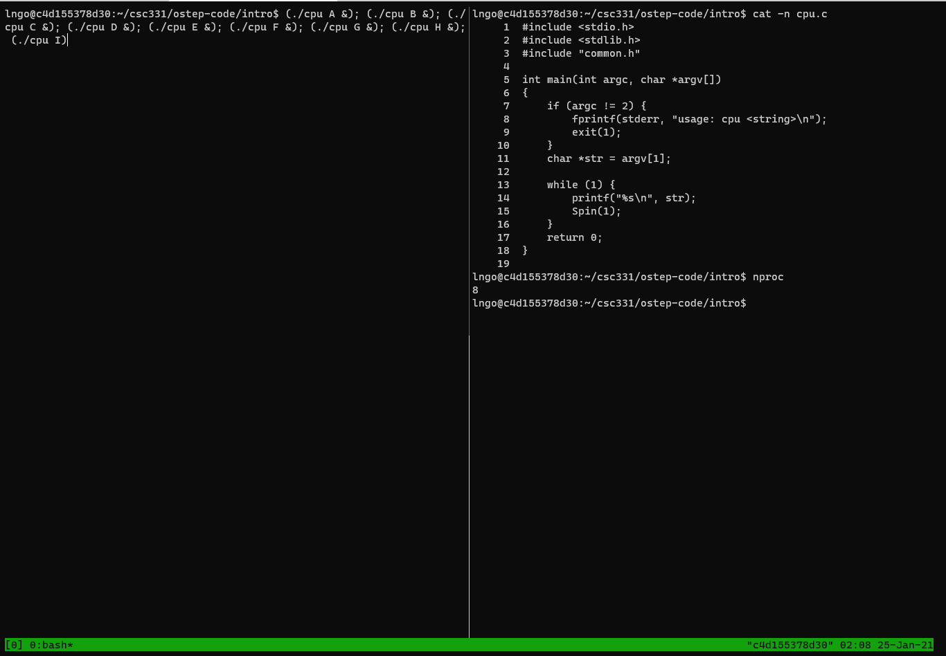
You can use Ctrl-b then the left and right arrows to move the active cursors between the two panes.

Move the cursor to the right channel and run the following commands to view the source code of cpu.c.

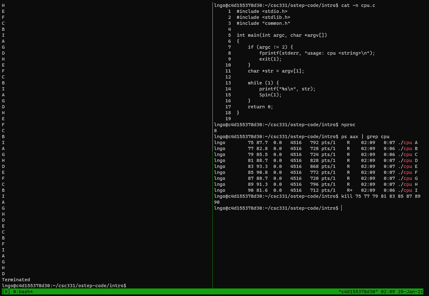
Also run nproc in the right pane to figure out how many CPUs your container has access to.
$ cat -n cpu.c
$ nproc
Run the following command on the left pane to execute cpu program accordingly.

Reminder: use Ctrl-b then the left and right arrows to move the active cursors between the two panes.

In my case, I have 8 cores, so my commands will be extended for two more.
$ (./cpu A &); (./cpu B &); (./cpu C &); (./cpu D &); (./cpu E &); (./cpu F &); (./cpu G &); (./cpu H &); (./cpu I)
To stop the running processes on the left pane, move to the right pane and running the following commands:
$ ps aux | grep cpu
Identify the process ID (the second columns), then use the kill to kill all the process IDs (see figure below).

7. The illusion of infinite CPU resources

A limited number of physical CPUs can still be represented as infnite number of CPUs through virtualization.

The OS will manage the scheduling and allocation of the actual run on physical resources.

8. Hands-on: Memory Virtualization

Type exit and hit Enter once to close one pane.

Type exit and hit Enter again to close tmux.

Run the following commands:
$ setarch `uname -m` -R /bin/bash
$ tmux
Press Ctrl-b and then Shift-% to split the tmux screen into two vertical panes again.

In the right pane, run the following command:
$ cat -n mem.c
In the left pane, run the following command:
$ (./mem 100 &); (./mem 200)
When finished, kill the two memory processes using the kill command and the process ID shown in the parentheses. You should switch to the right pane for this task.

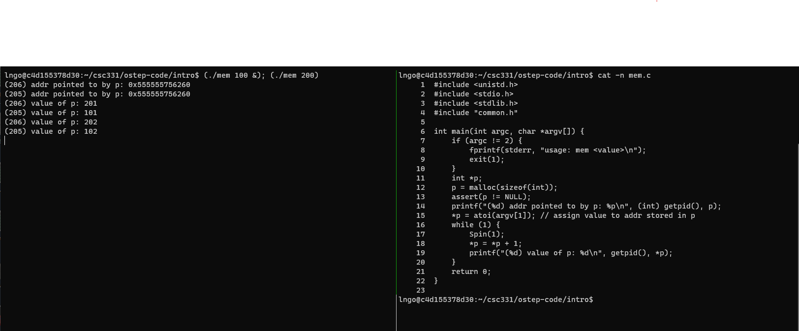
9. Do programs running concurrently occupy the same memory locations (addresses)?

Answer

No

10. The illusion of dedicated memory resources

Many running program share the physical memory space.

Each runnning program is presented with the illusion that they have access to their own private memory. This is called virtual address space, which is mapped to physical memory space by the OS.

Making memory references within one running program (within one’s own virtual address space) does not affect the private virtual address space of others.

Without the setarch command, the location of variable p will be randomize within the virtual address space of a process. This is a security mechanism to prevent others from guessing and applying direct manipulation techniques to the physical memory location that acually contains p.

11. Concurrency

As shown in CPU Virtualization and Memory Virtualization examples, the OS wants to manage many running programs at the same time.

This is called concurrency, and it leads to a number of interesting challenges in designing and implementing various management mechanisms within the OS.

12. Hands-on: Concurrency

Run clear command on both panes to clear the screen.

On the right pane, run the followings:
$ cat -n threads.c
On the left pane, run the following commands several times:
$ ./threads 50
$ ./threads 100
$ ./threads 200
threads.c creates two functions running at the same time, within the same memory space of the main program.

A single global variable named counter is being increased by both functions, thus the final value of counter should be twice that of the command line argument.

Now run with bigger values.
$ ./threads 20000
$ ./threads 30000
$ ./threads 30000
$ ./threads 30000

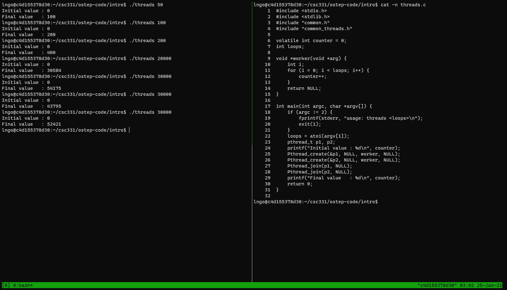
13. Observation

Naive concurrency gives you wrong results.

Naive concurrency gives you wrong and inconsistent results.

14. Why does this happen?

At machine level, incrementing counter involves three steps:

Load value of counter from memory into register,

Increment this value in the register, and

Write the value of counter back to memory.

What should have happened:

One thread increments counter (all three steps), then the other thread increments counter, now with the updated value.

What really happened:

One thread increments counter.

While this thread has not done with all three steps, the other thread steps in and attempts to increment the stale content of counter in memory.

15. Persistency

When the programs stop, everything in memory goes away: counter, p, str.

Physical components to store information persistently are needed.

Input/output or I/O devices:

Hard drives

Solid-state drives

Software managing these storage devices is called the file system.

Examples of system calls/standard libraries supporting the file system:

open()

write()

close()

16. A brief history of operating system research and development

A good paper to read: Hanser, Per Brinch. “The evolution of oeprating systems” 2001

17. Early operating systems: just libraries

Include only library for commonly used functions.

One program runs at a time.

Manual loading of programs by human operator.

18. Beyond libraries: protection

System calls

Hardware privilege level

User mode/kernel mode

trap: the initiation of a system call to raise privilege from user mode to kernel mode.

19. The era of multiprogramming

Minicomputer

multiprogramming: multiple programs being run with the OS switching among them.

Memory protection

Concurrency

20. The modern era

Personal computer

DOS: the Disk Operating System

Mac OS

Multics (MIT) -> UNIX (Bell Labs) -> BSD (Berkeley) -> Sun OS/Linux

Key Points

User programs are presented with uniform abstractions through the concept of virtualization.

Operating systems manage resources and map them to their corresponding virtualization abstractions.

Abstraction: The process

Overview

Teaching: 0 min
Exercises: 0 min

Questions

What is a program and what is a process?

Objectives

Understand the differences between a program and a process.

Know the possible states of a process.

What is a program?

A program is a static list of intsructions and data.

When a program runs, the OS takes this list and asks the CPU to execute them.

If we only have one CPU, how can we run more than one program at a time.

What is a process?

A process is a running program.

But the program itself is not running …

A process is an abstraction provided by the OS to describe the running of a program.

What is a process made of?

Memory that the process (running program) can address.

Memory registers.

Program counter.

Stack pointer.

Frame pointer.

I/O devices.

Process API

The operating system provides an API to help managing processes. Minimally, the followings are provided:

Create: an OS must have some methods to create new processes to run programs.

Destroy: interface to destroy process forcefully.

Wait: temporarily pausing the process.

Miscellaneous Control: suspend and resume processes.

Status: provide status about the state of the process.

Program counter.

Stack pointer.

Frame pointer.

I/O devices.

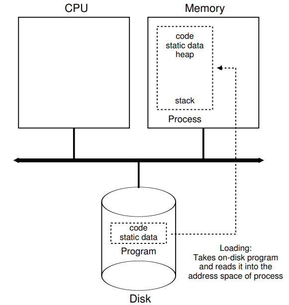
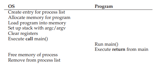
Process creation

When a program is run, the OS performs the following steps:

Load a program’s code and static data into memory (the virtual address space of the process).

Allocate memory for run-time stack (for stack).

Allocate memory for heap (used for dynamic memory allocation via malloc family).

Initialization:

File descriptor for standard input.

File descriptor for standard output.

File descriptor for error.

In Linux, everything is a file.

Begin executing from main().

Loading: from program to process

Process states

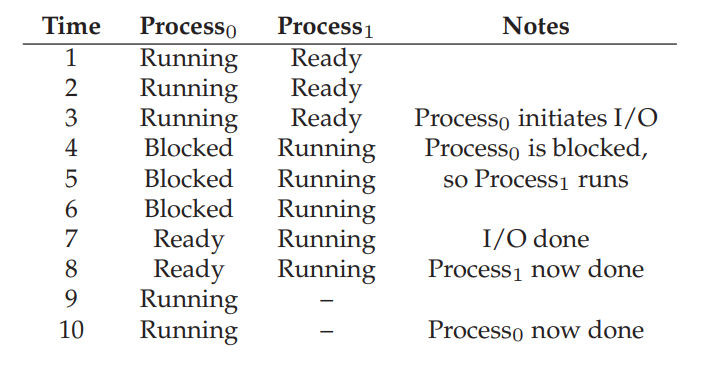
A process can be in one of the three states.

Running: the CPU is executing a process’ instructions.

Ready: the process is ready to run, but the OS is not running the process at the moment.

Blocked: the process has to perform some operation (e.g., I/O request to disk) that makes it not ready to run.

Process: state transition

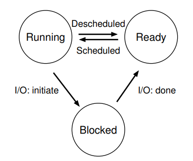
Process: state transition

When a process moves from ready to running, this means that it has been scheduled by the OS.

When a process is moved from running to ready, this means that it has been descheduled by the OS.

When an I/O request (within the process) is initiated, the running process become blocked by the OS until the I/O request is completed. Upon receiving the I/O completion signal, the OS moves the process’ state from blocked to ready, to wait to be scheduled by the OS.

Process: data structure

The OS is a program, and will data structures to track different pieces of information. that it has been scheduled by the OS.

How does the OS track the status of processes?

process list for all processes.

additional information for running process.

status of blocked process. from blocked to ready, to wait to be scheduled by the OS.

Example: xv6

Educational OS developed and maintained by MIT since 2006.

xv6 Git repository

Register contexts and status definition for a process

Example: Linux

Task struct in Linux: Lines 631-1329

Register contexts defined for each process: Line 267-312

[x86 CPU architecture model][https://en.wikibooks.org/wiki/X86_Assembly/X86_Architecture]

Key Points

A program is a static list of commands. When OS executes (runs) a program, the entire running operation is called a process.

Process API

Overview

Teaching: 0 min
Exercises: 0 min

Questions

How do you programmatically interact with processes?

Objectives

Knowing the usage of fork, exec, and wait.

1. Process API

Include three function calls:

fork()

exec()

wait()

2. fork()

… is a system call.

… is used to create a new process.

Documentation for fork()

Some important points:

fork() creates a new process by duplicating the calling process. The new process is referred to as the child process. The calling proces is referred to as the parent process.

The child process and the parent process run in separate memory spaces. At the time of fork() both memory spaces have the same content.

The child process is an exact duplicate of the parent process except for the following points:

The child has its own unique process ID, and this PID does not match the ID of any existing process group (setpgid(2)) or session.

The child’s parent process ID is the same as the parent’s process ID.

The child does not inherit outstanding asynchronous I/O operations from its parent (aio_read(3), aio_write(3)), nor does it inherit any asynchronous I/O contexts from its parent (see io_setup(2)).

The child inherits copies of the parent’s set of open file descriptors. Each file descriptor in the child refers to the same open file description (see open(2)) as the corresponding file descriptor in the parent. This means that the two file descriptors share open file status flags, file offset, and signal-driven I/O attributes.

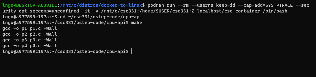
3. Hands-on: Getting started

Open a terminal (Windows Terminal or Mac Terminal).

Run the command to launch the image container for your platform:

Windows:
$ podman run --rm --userns keep-id --cap-add=SYS_PTRACE --security-opt seccomp=unconfined -it -v /mnt/c/csc331:/home/$USER/csc331:Z localhost/csc-container /bin/bash
Mac:
$ docker run --rm --userns=host --cap-add=SYS_PTRACE --security-opt seccomp=unconfined -it -v /Users/$USER/csc331:/home/$USER/csc331:Z csc-container /bin/bash
Navigate to /home/$USER/csc331

Change to directory ostep-code/cpu-api, then run make to build the programs.
$ cd ~/csc331/ostep-code/cpu-api
$ make

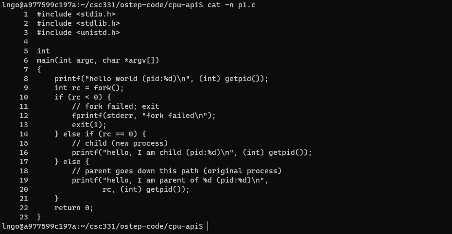
4. Hands-on: process creation using fork()
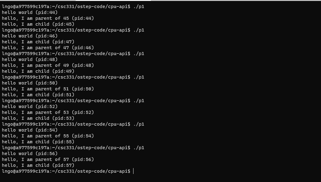
$ cat -n p1.c
Line 5-6: No idea why the author sets up the source code that way …

Line 8: prints out hello world and the process identifier (pid) of the current process.

Line 9: calls fork(), which initiate the creation of a new process. The return of this fuction call is assigned to variable rc.

Line 10: If rc is negative, the function call failed and the program exits with return value 1. This line is evaluated within the parent process (since the child process creation failed).

Line 14: If rc is non-negative

The fork call is successful, and you now have two process.

The new process is an almost exact copy of the calling process.

The new process does not start at main(), but begins immediately after fork().

The value of rc differs in each process.

The value of rc in the new process is 0.

The value of rc in the parent process is non-zero and actually is the pid of the new process.

Line 16 and line 19 confirms the above point by having the child process prints out its own process ID and the parent process prints out the rc value. These two values should be the same.

5. Hands-on: run p1

Run p1 several times.

What do you notice? - also see my screenshot

6. wait()/waitpid()/waitid()

… belongs to a family of system calls.

… are used to make a process to wait for its child process.

Documentation for wait()

Some important points:

What are we waiting for? state changes.

The child process was stopped by a signal.

The child process terminated.

The child process was resumed by a signal.

wait(): suspends execution of the calling thread until one of its child processes terminates.

7. Hands-on: processes management using wait()
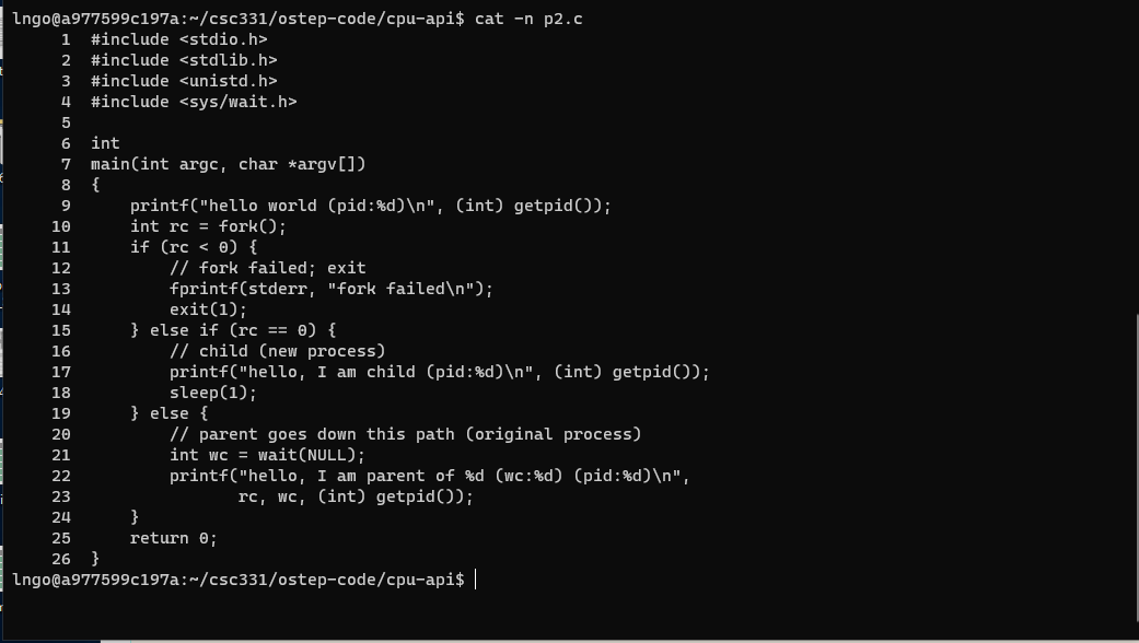
$ cat -n p2.c
Line 1-4: Pay attention to the libraries included.

Line 6-7: No idea why the author sets up the source code that way …

Line 9: prints out hello world and the process identifier (pid) of the current process.

Line 10: calls fork(), which initiate the creation of a new process. The return of this fuction call is assigned to variable rc.

Line 11: If rc is negative, the function call failed and the program exits with return value 1. This line is evaluated within the parent process (since the child process creation failed).

Line 15: If rc is equal to 0.

The child process will execute the codes inside this conditional block.

Line 17: prints out a statement and the child’s pid.

Line 18: sleeps for one second.

Line 19: This is the parent process (rc is non-negative and not equal to 0)

Line 21: calls the wait() function.

Line 22: prints out the information of the parent process.

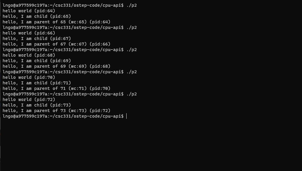
8. Hands-on: run p2

Run p2 several times.

What do you notice about the runs?

9. exec()

Documentation for exec()

fork() lets you create and run a copy of the original process.

exec() lets you run a different process in place of the copy of the original process.

10. Hands-on: processes management using exec()
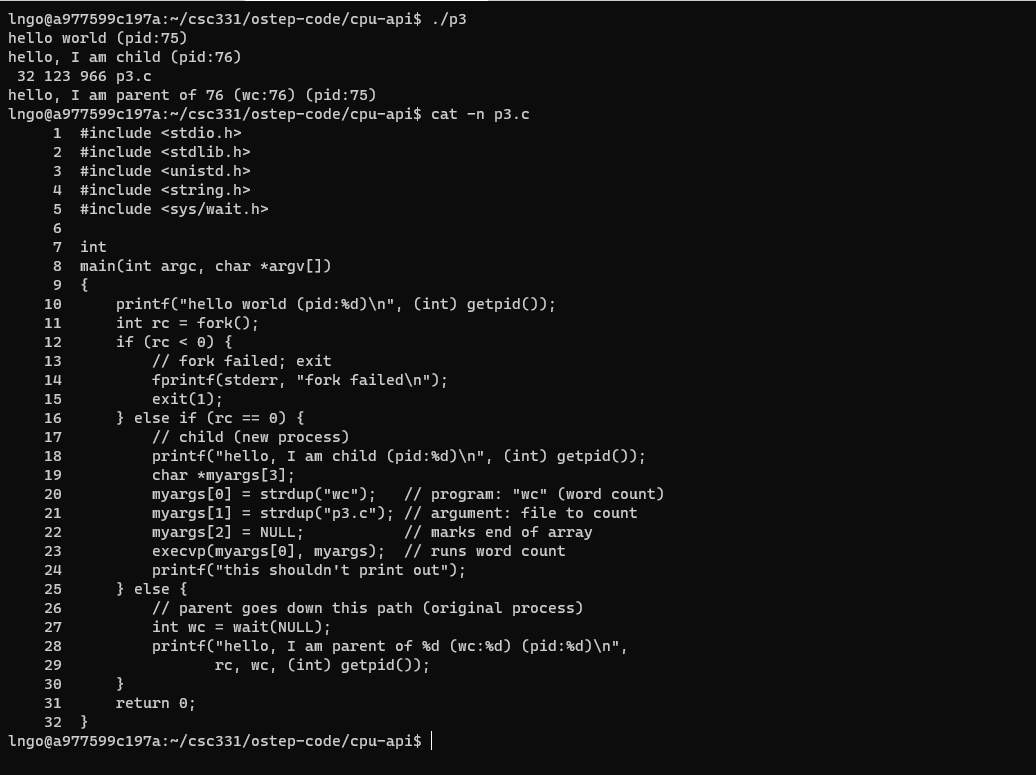
$ ./p3
$ cat -n p3.c
Line 1-5: Pay attention to the libraries included.

Line 7-8: main

Line 10: prints out hello world and the process identifier (pid) of the current process.

Line 11: calls fork(), which initiate the creation of a new process. The return of this fuction call is assigned to variable rc.

Line 12: If rc is negative, the function call failed and the program exits with return value 1. This line is evaluated within the parent process (since the child process creation failed).

Line 16: If rc is equal to 0.

The child process will execute the codes inside this conditional block.

Line 18: prints out a statement and the child’s pid.

Line 19-22: sets up parameters for a shell command (wc in this case).

Line 23: exec replaces the current child process with a completely new process to execute the wc command.

Line 24: This line’s code is contained in the current child process, but was wiped out when exec replaces the current child process with the new process for wc.

Line 25: This is the parent process (rc is non-negative and not equal to 0)

Line 27: calls the wait() function.

Line 28: prints out the information of the parent process.

11. Why fork(), wait(), and exec()?

The separation of fork() and exec() is essential to the building of a Linux shell.

It lets the shell runs code after the call to fork(), but before the call to exec().

This facilitates a number of interesting features in the UNIX shell.

12. The Shell

What is the UNIX shell?.

In Unix, the shell is a program that interprets commands and acts as an intermediary between the user and the inner workings of the operating system. Providing a command-line interface (that is, the shell prompt or command prompt), the shell is analogous to DOS and serves a purpose similar to graphical interfaces like Windows, Mac, and the X Window System.

13. The Shell

What is the UNIX shell?.

In Unix, the shell is a program …

The Shell

In Unix, the shell is a program …

Therefore, the running shell is a process.

In other words, inside a running shell, if we want to run another program, we are essentially asking a process (the running shell) to create and run another process.

14. When you run a program from the shell prompt …

The shell will

find out where the program is in the file system.

call fork() to create a new child process (to run the program).

call one of the exec() family functions in the scope of this child process to actually load and run this program.

call wait() to wait for the child process to finish (now with new process content) before giving user the shell prompt again.

15. When you run a program from the shell prompt …

The shell will

find out where the program is in the file system.

call fork() to create a new child process (to run the program).

call one of the exec() family functions in the scope of this child process to actually load and run this program.

call wait() to wait for the child process to finish (now with new process content) before giving user the shell prompt again.

16. Hands-on 7: redirection
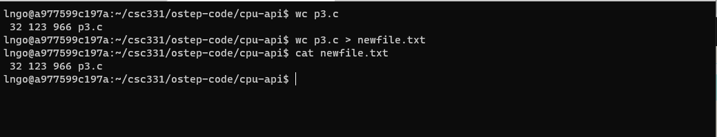
$ wc p3.c
$ wc p3.c > newfile.txt
$ cat newfile.txt
The shell …

finds out where wc is in the file system.

prepares p3 as in input to wc.

calls fork() to create a new child process to run the command.

recognizes that > represents a redirection, thus closes the file descriptor to standard output and replaces it with a file descriptor to newfile.txt.

calls one of exec() family to run wc p3.c.

output of wc p3.c are now send to newfile.txt.

calls wait() to wait for the child process to finish before giving user the prompt again.

17. Hands-on 8: more on file descriptors
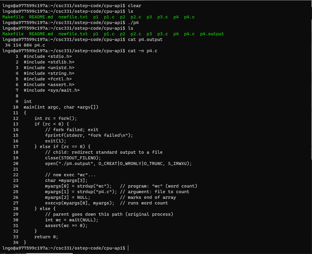
$ ls
$ ./p4
$ ls
$ cat p4.output
$ cat -n p4.c
wc p4 should have printed out to terminal.

close(STDOUT_FILENO) closes the file descriptor that writes to the terminal (hence free up that particular file descriptor ID).

open(“./p4.output”, …) creates a file descriptor for the p4.output file, but since the file descriptor ID for the terminal is now free, this file descriptor is assigned to p4.output.

As wc p4 is executed and attempts to write to terminal, it actually writes to p4.output instead.

Hands-on 9: piping

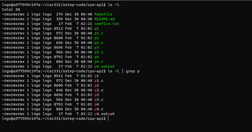
$ ls -l
$ ls -l | grep p

Piping

Other system calls …

kill(): send signals to a process, including directive to pause, die, and other imperatives.

http://man7.org/linux/man-pages/man2/kill.2.html

SIGINT: signal to terminate a process

SIGTSTP: pause the process (can be resumed later).

signal(): to catch a signal.

http://man7.org/linux/man-pages/man7/signal.7.html

Key Points

Through fork, exec, and wait, processes can be controlled and manipulated.

Limited Direct Execution

Overview

Teaching: 0 min
Exercises: 0 min

Questions

How to efficiently virtualize the CPU with control?

Objectives

First learning objective. (FIXME)

1. CPU virtualization recall

To support the illusion of having multple processes running concurrently on a single physical CPU, we can have the CPU run one process for a while, then run another, and so on.

This is called time sharing.

2. Design goals of CPU virtualization

Performance

The process can be itself and run as fast as possible without frequent interaction with the OS.

Control

We want to avoid the scenario where a process can run forever and take over all the machine’s resources or a process performs unauthorized actions. This requires interaction with the OS.

3. The question!

How to efficiently virtualize the CPU with control?

4. Efficient

The most efficient way to execute a process is through direct execution.

Problem!

Once the program begins to run, the OS becomes a complete outsider.

No control over the running program.

Problem 1: The program can access anything it wants to, including restricted operations (direct access to hardware devices, especially I/O for unauthorized purposes).

Problem 2: The program may never switch to a different process without explicit. instructions in main(), thus defeating the purposes of time-sharing.

5. Problem: working with restricted operations

The process should be able to perform restricted operations, such as disk I/O, open network connections, etc.

But we should not give the process complete control of the system.

Rephrase: The process should be able to have its restricted operations performed.

Solution: hardware support via processor modes

User mode

Kernel mode

6. Process modes

A mode bit is added to hardware to support distinguishing between user mode and kernel mode.

Some instructions are designated as privileged instructions that cannot be run in user mode (only in kernel mode).

A user-mode process trying to perform privileged instructions will raise a protection fault and be killed.

How can these instructions be called by a process in user-mode?

System calls

7. System calls

A small set of APIs for restricted operations.

XV6 system calls

Linux x86_64 has 335 systems called (0 to 334) - Last commit June 2, 2018.

Linux uses a sys_call_table to keep the syscall handlers.

Syscall_64.tbl

These system calls enable user-mode process to have restricted operations performed without having to gain complete control over the system.

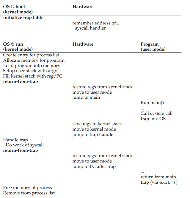
8. How does a system call happen?

To make a system call, the process need to switch from user mode to kernel mode, do the privileged operation, and then switch back.

This is done through hardware support

Require assembly instructions

trap: go from user mode to kernel mode.

return-from-trap: go back from kernel mode to user mode.

9. System calls versus normal C calls?

Function declarations are the same

System calls

Have trap instruction in them

have extra level of indirection (movements between modes).

perform restricted operations

have bigger overhead and are slower than equivalent function calls.

can use kernel stack.

10. Names of system calls

User space definition:

libc’s definition for write()

Kernel definition:

Linux definition for write()

The user space definition will eventually call the kernel definition.

11. Problem: switching processes

A free running process may never stop or switch to another process.

OS needs to control the process, but how?

Once a process is running, OS is NOT running (OS is but another process)

The question: How can OS regain control of the CPU from a process so that it can switch to another process?

12. First approach: cooperative processes

All programmers promise to insert yield() into their code to give up CPU resources to other people’s program.

We have solved the problem and achieved eternal world peace.

Even in a perfect world, what happens if a process falls into an infinite loop prior to calling yield()?

Collaborative multitasking (Windows 3.1X, Mac PowerPC)

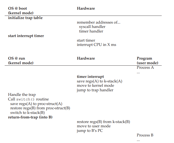
13. Second approach: non-cooperative processes

Similar to processor modes, the hardware once again provided assistance via timer interrupt.

A timer device can be programmed to raise an interrupt periodically.

When the interrupt is raised, the running process stops, a pre-configured interrupt handler in the OS runs.

The OS regains control.

14. Second approach: non-cooperative processes

The OS first decides which process to switch to (with the help from the scheduler).

The OS executes a piece of assemble code (context switch).

Save register values of the currently running process into its kernel stack.

Restore register values of the soon running process from its kernel stack.

Key Points

virtualization of the CPU must be done in an efficient manner. At the same time, the OS must retain control over the system. This is accomplished by combining user/kernel modes, trap table, timer interrupt, and context switching.

CPU Scheduling

Overview

Teaching: 0 min
Exercises: 0 min

Questions

How can an illusion of infinite CPU be managed?

Objectives

Understand the assumptions behind FCFS/SJF

Understand the reasoning behind MLFQ rules

1. What is CPU scheduling?

The allocation of processors to processes over time

Key to multiprogramming

Increase CPU utilization and job throughput by overlapping I/O and computation

Different process queues representing different process states (ready, running, block …)

Policies: Given more than one runnable processes, how do we choose which one to run next?

2. Initial set of simple assumptions

Each job (process/thread) runs the same amount of time.

All jobs arrive at the same time.

Once started, each job runs to completion (no interruption in the middle).

All jobs only use the CPU (no I/O).

The run time of each job is known.

These are unrealistic assumptions, and we will relax them gradually to see how it works in a real system.

3. First performance metric

Average turn around time of all jobs.

turn_around_time = job_completion_time - job_arrival_time

4. Algorithm 1: First Come First Server (FCFS/FIFO)

First Come First Server (FCFS)/ First In First Out (FIFO)

Job Arrival Time Service Time

A 0 3

B 0 3

C 0 3

For FCFS, jobs are executed in the order of their arrival.

When jobs with same arrival time arriva, let’s assume a simple alphabetic ordering based on jobs’ names.

Job	Arrival Time	Service Time
A	0	3
B	0	3
C	0	3

5. FCFS/FIFO in action

0 1 2 3 4 5 6 7 8 9 10 11

A A A

B B B

C C C

Average_turn_around_time = (3 + 6 + 9) / 3 = 6.

6. Initial set of simple assumptions

~~Each job (process/thread) runs the same amount of time.~~

All jobs arrive at the same time.

Once started, each job runs to completion (no interruption in the middle).

All jobs only use the CPU (no I/O).

The run time of each job is known.

7. Algorithm 1: First Come First Server (FCFS/FIFO)

Job Arrival Time Service Time

A 0 8

B 0 3

C 0 3

For first come first server, jobs are executed in the order of their arrival.

When jobs with same arrival time arriva, let’s assume a simple alphabetic ordering based on jobs’ names.

Job	Arrival Time	Service Time
A	0	8
B	0	3
C	0	3

8. FCFS/FIFO in action

0 1 2 3 4 5 6 7 8 9 10 11 12 13 14 15

A A A A A A A A

B B B

C C C

Average_turn_around_time = (8 + 11 + 14) / 3 = 11.

9. Algorithm 2: Shortest Job First (SJF)

Job Arrival Time Service Time

A 0 8

B 0 3

C 0 3

For SJF, jobs are executed in the order of their arrival.

When jobs with same arrival time arriva, jobs with shorter service time are executed first.

Job	Arrival Time	Service Time
A	0	8
B	0	3
C	0	3

10. SJF in action

0 1 2 3 4 5 6 7 8 9 10 11 12 13 14 15

B B B

C C C

A A A A A A A A

Average_turn_around_time = (3 + 6 + 14) / 3 = 7.67.

11. Initial set of simple assumptions

~~Each job (process/thread) runs the same amount of time.~~

~~All jobs arrive at the same time.~~

Once started, each job runs to completion (no interruption in the middle).

All jobs only use the CPU (no I/O).

The run time of each job is known.

12. Algorithm 1: FCFS/FIFO

Job Arrival Time Service Time

A 0 8

B 2 3

C 2 3

For FCFS, jobs are executed in the order of their arrival time.

When jobs with same arrival time arrive, let’s assume a simple alphabetic ordering based on jobs’ names.

Job	Arrival Time	Service Time
A	0	8
B	2	3
C	2	3

13. FCFS/FIFO in action

0 1 2 3 4 5 6 7 8 9 10 11 12 13 14 15

A A A A A A A A

B B B

C C C

Average_turn_around_time = (8 + 9 + 12) / 3 = 9.67.

B and C suffer from a long waiting time, but A already got the CPU.

14. Initial set of simple assumptions

~~Each job (process/thread) runs the same amount of time.~~

~~All jobs arrive at the same time.~~

~~Once started, each job runs to completion (no interruption in the middle).~~

All jobs only use the CPU (no I/O).

The run time of each job is known.

15. Preemptive vs Non-preemptive

Non-Preemptive Scheduling

Once the CPU has been allocated to a process, it keeps the CPU until it terminates or blocks.

Suitable for batch scheduling, where we only care about the total time to finish the whole batch.

Preemptive Scheduling

CPU can be taken from a running process and allocated to another (timer interrupt and context switch).

Needed in interactive or real-time systems, where response time of each process matters.

16. Algorithm 3: Shortest Time-to-Completion First (STCF)

Also known as Preemptive Shortest Job First (PSJF)

Job Arrival Time Service Time

A 0 8

B 2 3

C 2 3

For FCFS, jobs are executed in the order of their arrival time.

When jobs with same arrival time arrive, let’s assume a simple alphabetic ordering based on jobs’ names.

Job	Arrival Time	Service Time
A	0	8
B	2	3
C	2	3

17. STCF/PSJF in action

0 1 2 3 4 5 6 7 8 9 10 11 12 13 14 15

A A A A A A A A

B B B

C C C

Average_turn_around_time = (14 + 3 + 6) / 3 = 7.67.

18. Second performance metric

Average response time of all jobs.

The time from when the job arrives to when it is first scheduled.

response_time = first_scheduled_time - job_arrival_time

19. STCF/PSJF in action

0 1 2 3 4 5 6 7 8 9 10 11 12 13 14 15

A A A A A A A A

B B B

C C C

Average_response_time = (0 + 0 + 3) / 3 = 1

20. Algorithm 4: Round Robin (RR)

Job Arrival Time Service Time

A 0 8

B 2 3

C 2 3

All jobs are placed into a circular run queue.

Each job is allowed to run for a time quantum q before being preempted and put back on the queue.

Example: q=1

Job	Arrival Time	Service Time
A	0	8
B	2	3
C	2	3

21. RR in action

0 1 2 3 4 5 6 7 8 9 10 11 12 13 14 15

A A A A A A A A

B B B

C C C

Average_response_time = (0 + 0 + 1) / 3 = 0.33

22. Algorithm 4: Round Robin (RR)

The choice of q is important.

If q becomes infinite, RR becomes non-preemptive FCFS.

If q becomes 0, RR becomes simultaneously sharing of process (not possible due to context switching).

q should be a multiple of the timer interrupt interval

23. Initial set of simple assumptions

~~Each job (process/thread) runs the same amount of time.~~

~~All jobs arrive at the same time.~~

~~Once started, each job runs to completion (no interruption in the middle).~~

~~All jobs only use the CPU (no I/O).~~

The run time of each job is known.

24. (Almost) all processes perform I/O

When a job is performing I/O, it is not using the CPU. In other words, it is blocked waiting for I/O to complete.

It makes sense to use this time to run some other jobs.

25. Jobs with I/O

Job Arrival Time CPU Time I/O

A 0 5 One per 1 sec

B 0 5 none

Job	Arrival Time	CPU Time	I/O
A	0	5	One per 1 sec
B	0	5	none

26. Normal STCF treating A as a single job

0 1 2 3 4 5 6 7 8 9 10 11 12 13 14 15

A I/O A I/O A I/O A I/O A

B B B B B

Average_turn_around_time = (9 + 14) / 2 = 11.5

Average_response_time = (0 + 9) / 2 = 4.5

27. STCF treating A as 5 sub-jobs

0 1 2 3 4 5 6 7 8 9 10 11 12 13 14 15

A I/O A I/O A I/O A I/O A

B B B B B

Average_turn_around_time = (9 + 10) / 2 = 9.5

Average_response_time = (0 + 1) / 2 = 0.5

28. Initial set of simple assumptions

~~Each job (process/thread) runs the same amount of time.~~

~~All jobs arrive at the same time.~~

~~Once started, each job runs to completion (no interruption in the middle).~~

~~All jobs only use the CPU (no I/O).~~

~~The run time of each job is known.~~

The worst assumption:

Most likely never happen in real life

Yet, without it, SJF/STCF becomes invalid.

29. The question

How do we schedule jobs without knowing their run time duration so that we can minimize turn around time and also minimize response time for interactive jobs?

30. Multi-level Feedback Queue (MLFQ)

Invented by Fernando Jose Corbato (1926 - )

Ph.D. in Physics (CalTech)

MIT Professor

One of the original developers of Multics (Predecessor of UNIX)

First use of password to secure file access on computers.

Recipient of the 1990 Turing Award (The Nobel prize in computing)

31. Multi-level Feedback Queue (MLFQ)

Learn from the past to predict the future

Common in Operating Systems design. Other examples include hardware branch predictors and caching algorithms.

Works when jobs have phases of behavior and are predictable.

Assumption: Two categories of jobs

Long-running CPU-bound jobs

Interactive I/O-bound jobs

32. Multi-level Feedback Queue (MLFQ)

Consists of a number of distinct queues, each assigned a different priority level.

Each queue has multiple ready-to-run jobs with the same priority.

At any given time, the scheduler choose to run the jobs in the queue with the highest priority

If multiple jobs are chosen, run them in Round-Robin

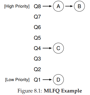
32. Multi-level Feedback Queue (MLFQ): Feedback?

Rule 1: If Priority(A) > Priority(B), A runs and B doesn’t

Rule 2: If Priority(A) == Priority(B), RR(A, B)

Does it work well?

33. Multi-level Feedback Queue (MLFQ): Feedback?

Rule 1: If Priority(A) > Priority(B), A runs and B doesn’t

Rule 2: If Priority(A) == Priority(B), RR(A, B)

With only these two rules, A and B will keep alternating via RR, and C and D will never get to run.

What other rule(s) do we need to add?

We need to understand how job priority changes over time.

34. Attempt 1: How to change priority?

Rule 3: When a job enter the system, it is placed at the highest priority (the top most queue).

Rule 4a: If a job uses up an entire time slice while running, its priority is reduced (it moves down one queue).

Rule 4b: If a job gives up the CPU (voluntarily) before the time slice is up, it stays at the same priority level.

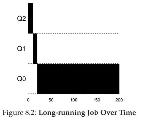
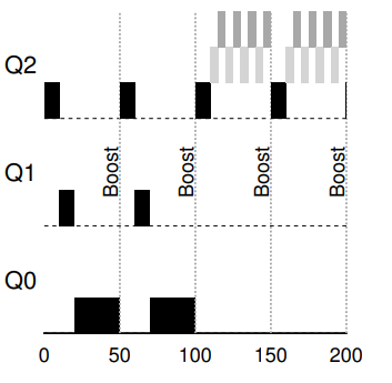
35. Example 1: A single long-running job

System maintains three queues, in the order of priority from high to low: Q2, Q1, and Q0.

Time-slice of 10 ms

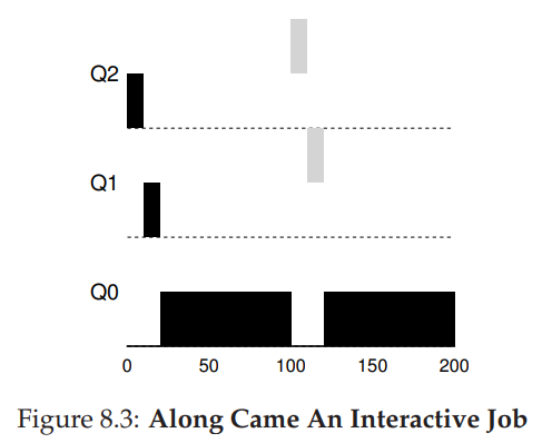
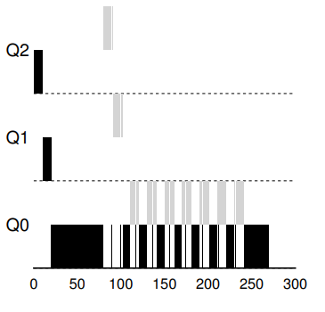
36. Example 2: Along came a short job

Job A (Dark): long-running CPU intensive

Job B (Gray): short-running interactive

Major goal of MLFQ: At first, since the scheduler does not know about the job, it first assumes that is might be a short job (higher priority). If it is not a short job, it will gradually be moved down the queues.

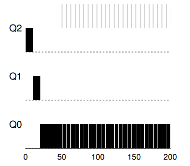
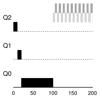
36. Example 3: What about I/O?

The interactive job (gray) only needs the CPU for 1 ms before performing an I/O. MLFQ keeps B at the highest priority before B keep releasing the CPU.

What are potentially problems?

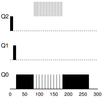
37. Problem 1: Starvation

If new interactive jobs keep arriving, long running job will stay at the bottom queue and never get any work done.

38. Problem 2: Gaming the system

What if some industrious programmers intentionally write a long running program that relinquishes the CPU just before the time-slice is up (Job B).

39. Problem 3: What if a program changes behavior?

Starting out as a long running job

Turn into an interactive job

39. Attempt 2: Priority boost

Rule 5: After some time period S, move all the jobs in the system to the topmost queue.

40. Problem: Starvation

Rule 5 help guaranteeing that processes will not be staved. It also helps with CPU-bound jobs that become interactive

41. What S should be set to?

Voodoo constants (John Ousterhout)

S requires some form of magic to set them correctly.

Too high: long running jobs will starve

Too low: interactive jobs will not get a proper share of the CPU.

42. Attempt 3: Better accounting

Rewrite of Rule 4 to address the issue of gaming the system.

Rule 5: Once a job uses up its time allotment at a given level (regardless of how many time it has given up the CPU), its priority is reduced.

43. Summary

Rule 1: If Priority(A) > Priority(B), A runs (B doesn’t)

Rule 2: If Priority(A) = Priority(B), RR(A, B)

Rule 3: When a job enter the system, it is placed at the highest priority (the top most queue).

Rule 4: Once a job uses up its time allotment at a given level (regardless of how many time it has given up the CPU), its priority is reduced.

Rule 5: After some time period S, move all the jobs in the system to the topmost queue.

MLFQ observes the execution of a job and gradually learns what type of job it is, and prioritize it accordingly.

Excellent performance for interactive I/O bound jobs: good response time.

Fair for long-running CPU-bound jobs: good turnaround time without starvation.

Used by many systems, including FreeBSD, MacOS X, Solaris, Linux 2.6, and Windows NT

Key Points

FCFS/SJF operates based on a set of assumptions that are unrealistics in the real world.

MLFQ rules provide an adaptive approach to adjust the scheduling as needed.

GDB Debugger

Overview

Teaching: 0 min
Exercises: 0 min

Questions

Debugging C program the hard way!

Objectives

First learning objective. (FIXME)

1. In a nutshell

Developed in 1986 by Richard Stallman at MIT.

Current official maintainers come from RedHat, AdaCore, and Google.

Significant contribution from the open source community.

2. Brief Technical Details

Allows programmers to see inside and interact/modify with all components of a programs, including information inside the registers.

Allows programmers to walk through the program step by step, including down to instruction level, to debug the program.

3. Cheatsheet

Study this cheatsheet

Developed by Dr. Doeppner at Brown University.

Become very comfortable with terminal!

We will work on the terminal extensively here, say goodbye to VSCode. You can certainly use VSCode, but you will miss out on a fine tool!

4. tmux

Our workspace is limited within the scope of a single terminal (a single shell) to interact with the operating system.

tmux: terminal multiplexer.

tmux allows user to open multiple terminals and organize split-views (panes) within these terminals within a single original terminal.

We can run/keep track off multiple programs within a single terminal.

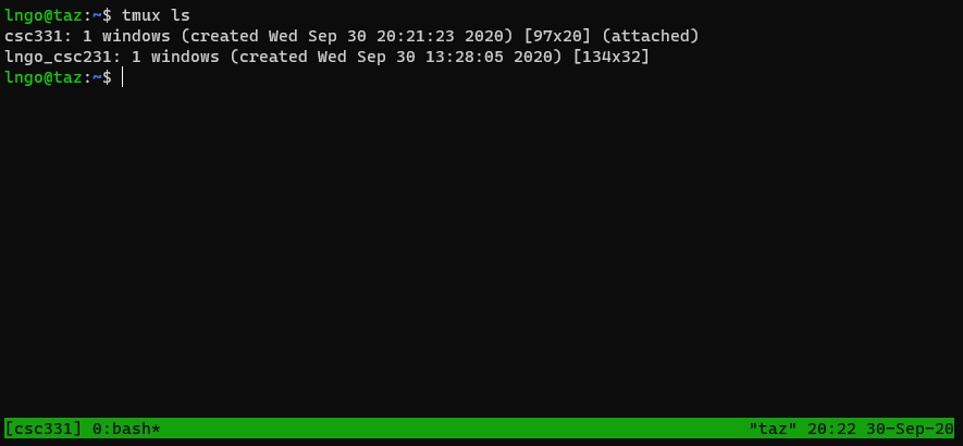
5. tmux quickstart 1: multiple sessions

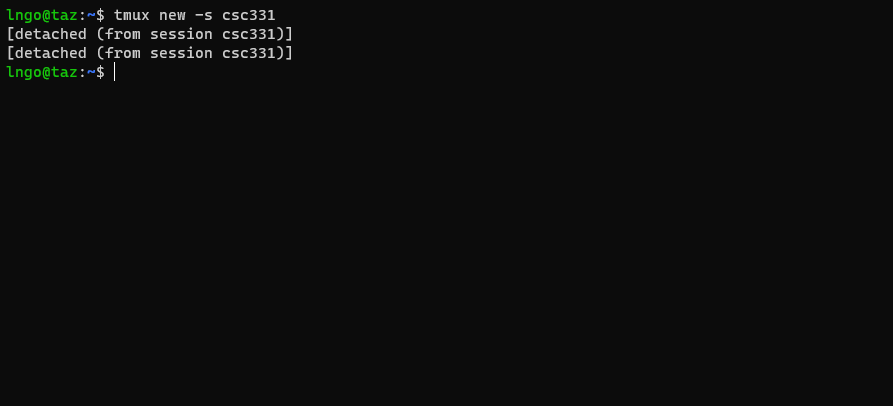
Start new with a session name: tmux new -s csc331

You are now in the new tmux session.

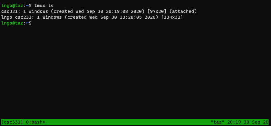
List sessions: tmux ls

To go back to the main terminal, press Ctrl-b, then press d.

To go back into the csc331 session: tmux attach-session -t csc331.

To kill a session:

From inside the session: exit

From outside the session: tmux kill-session -t csc331

6. Hands on: navigating among multiple tmux sessions

Run tmux ls to check and tmux kill-session to clean up all existing tmux sessions.

Create a new session called s1.

Detach from s1 and go back to the main terminal.

Create a second session called s2.

Detach from s2, go back to the main terminal, and create a third session called s3.

Use tmux ls to view the list of tmux sessions.

Navigate back and forth between the three sessions several times.

Kill all three sessions using only exit!

SCREENSHOT

7. tmux quickstart 2: multiple panes

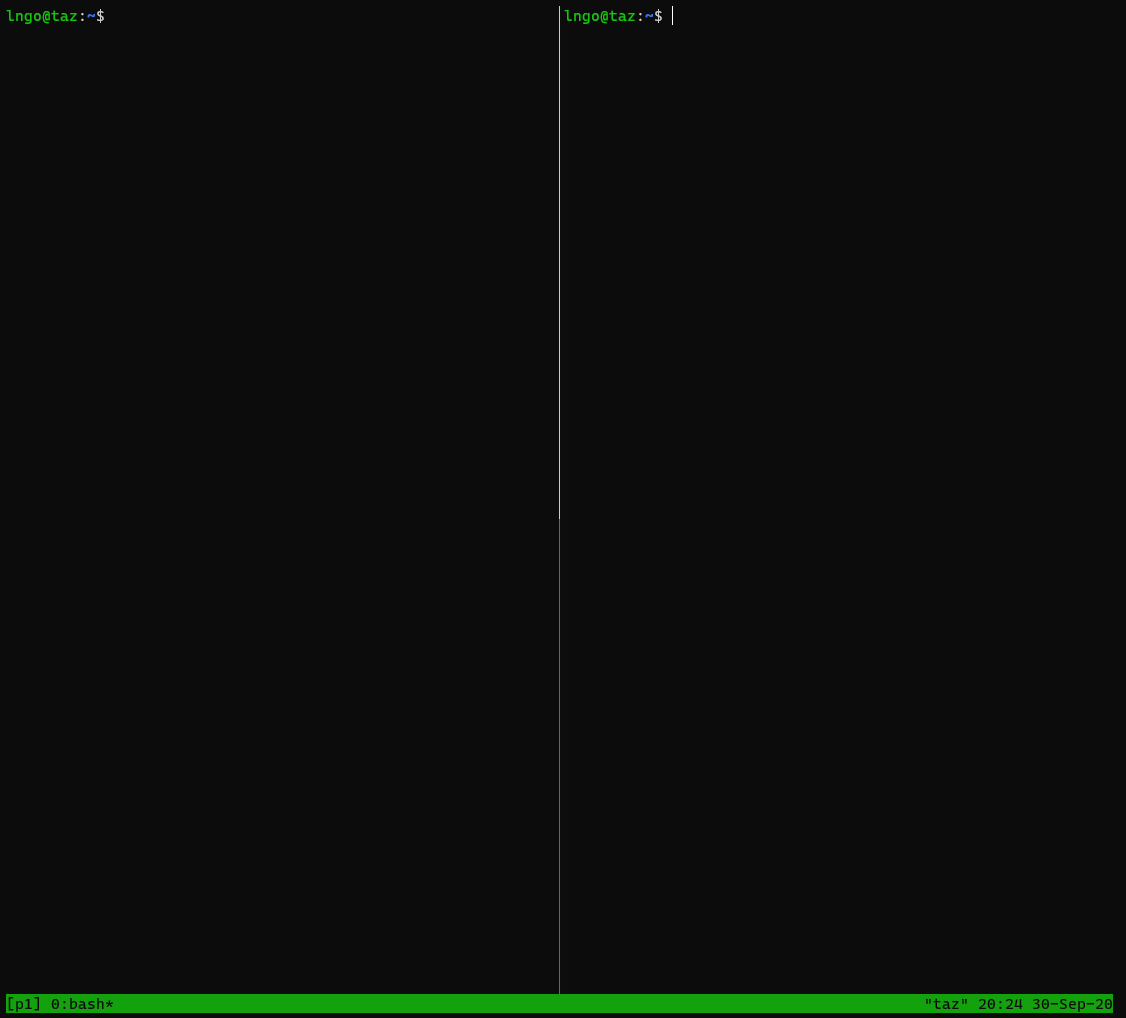
Create a new session called p1.

Splits terminal into vertical panels: Ctrl-b then Shift-5 (technical documents often write this as Ctrl-b and %).

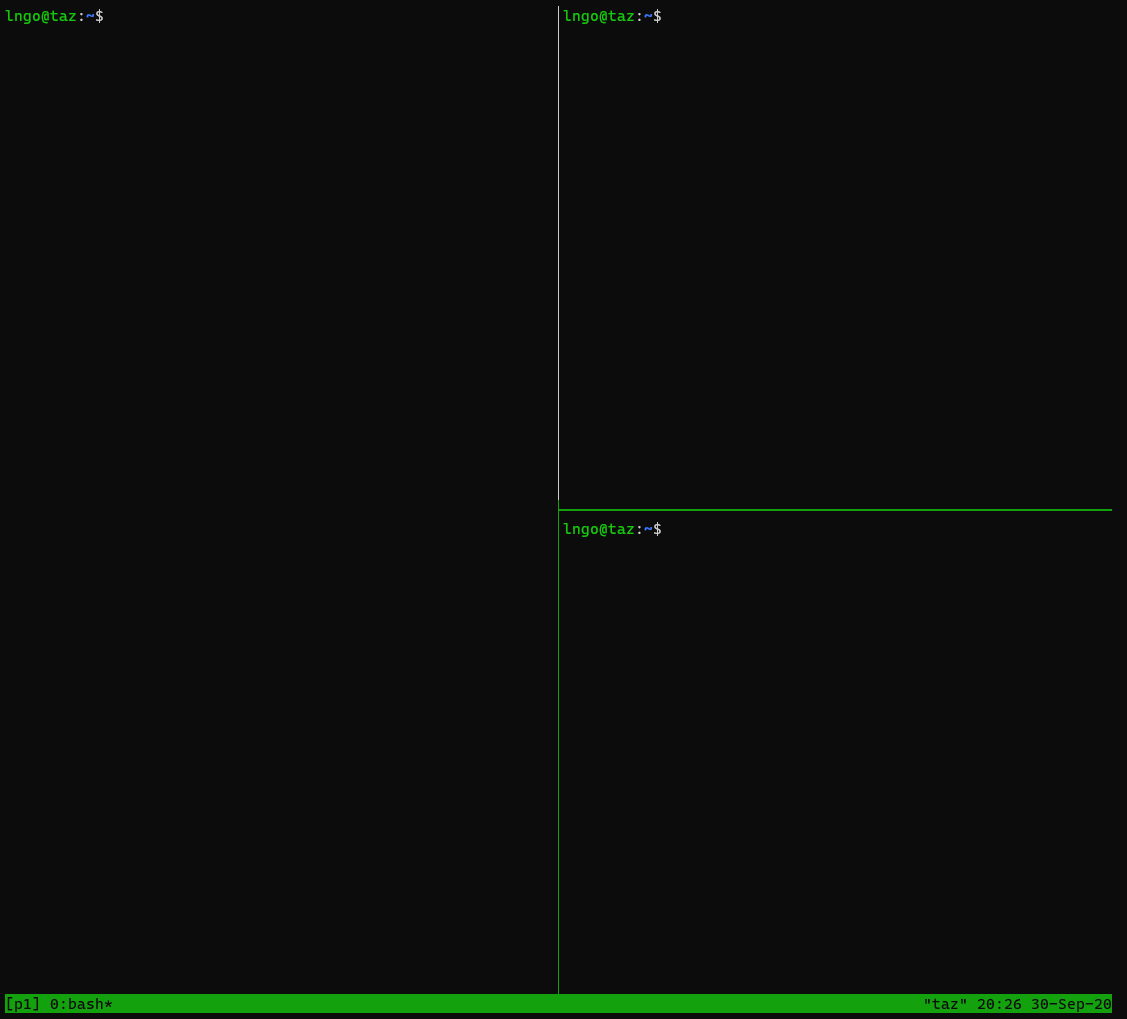
Splits terminal (the current pane) into horizontal panels: Ctrl-b then Shift-' ( technical documents often write this as Ctrl-b and ").

Toggle between panels: Ctrl-b then Space.

To move from one panel to other directionally: Ctrl-bthen the corresponding arrow key.

Typing exit will close one pane.

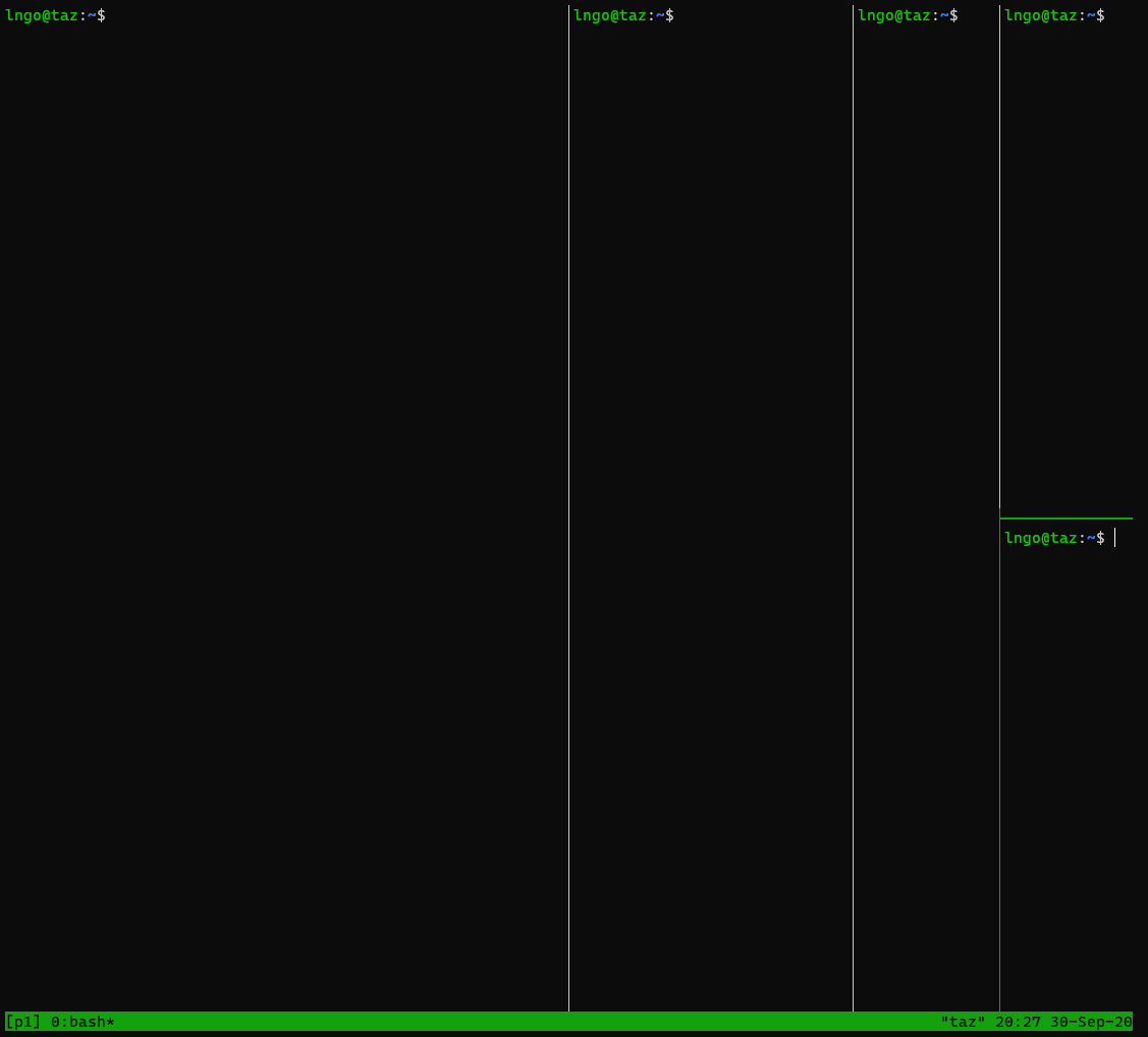
8. Hands on: creating multiple panes

Run tmux ls to check and tmux kill-session to clean up all existing tmux sessions.

Create a new session called p1.

Organize p1 such that:

p1 has four vertical panes.

The last vertical pane of p1 has three internal horizontal panes.

Kill all panes using exit!

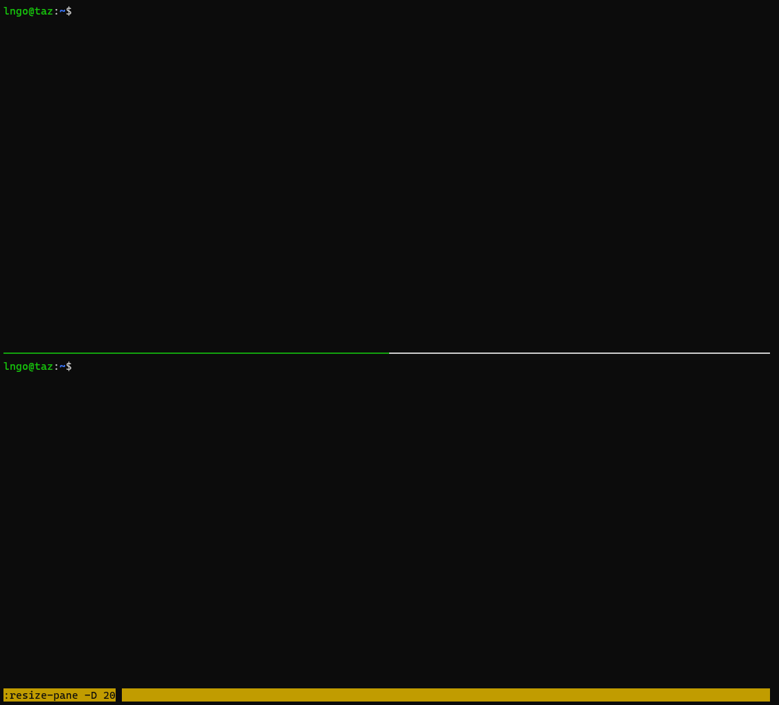
9. tmux quickstart 3: resizing

What we did in Hands-on 8 was not quite usable.

We need to be able to adjust the panes to the proper sizes.

This can be done by issuing additional commands via tmux’s command line terminal.

Run tmux ls to check and tmux kill-session to clean up all existing tmux sessions.

Create a new session called p1.

Split the session horizontally.

Move the active cursor to the top pane.

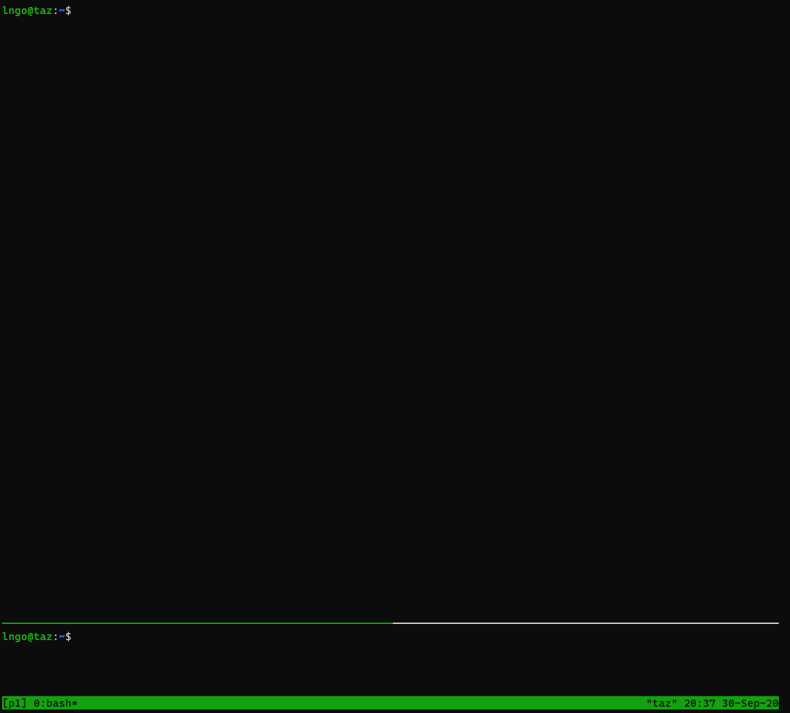
Open tmux command by typing Ctrl-b then Shift-;

Use the following command for resizing the current pane down:

resize-pane -D 20: (Resizes the current pane down by 20 cells)

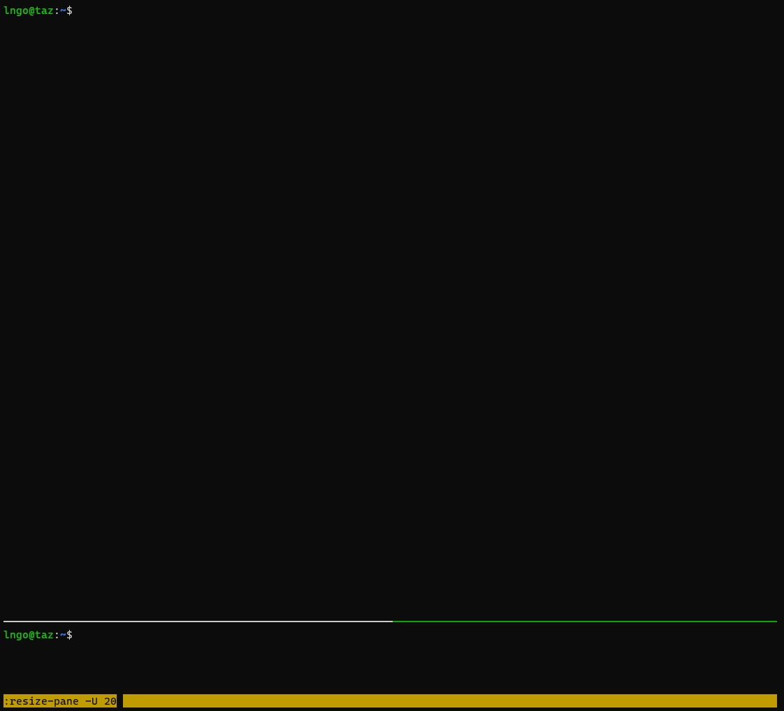
Move the active cursor to the bottom pane.

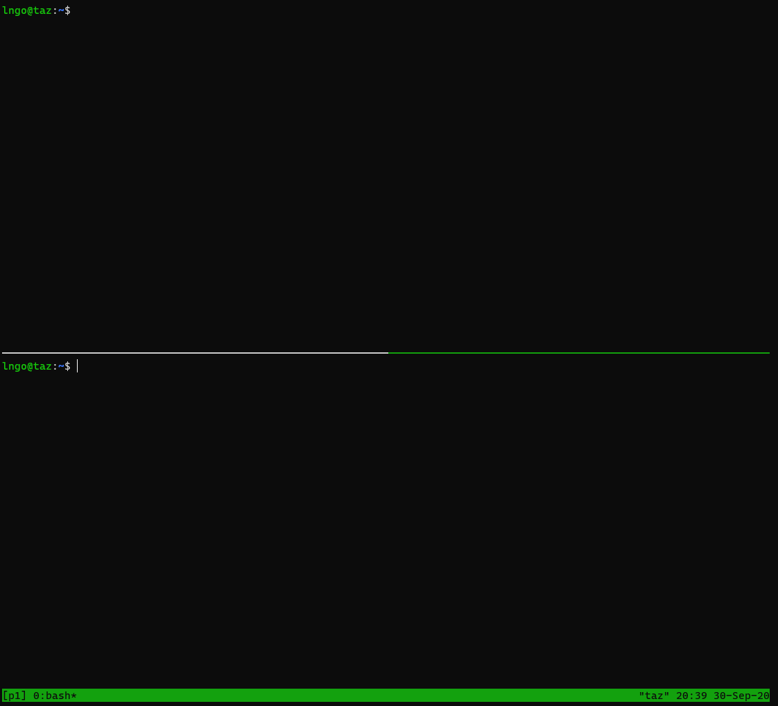
Open tmux command by typing Ctrl-b then Shift-;

Use the following command for resizing the current pane down:

resize-pane -U 20: (Resizes the current pane up by 20 cells)

10. Hands on: creating multiple panes

Run tmux ls to check and tmux kill-session to clean up all existing tmux sessions.

Create a new session called p1.

Split p1 once vertically.

Use the following commands to resize the left pane:

resize-pane -L 20 (Resizes the current pane left by 20 cells)

resize-pane -R 20 (Resizes the current pane right by 20 cells)

12. Setup an application with gdb

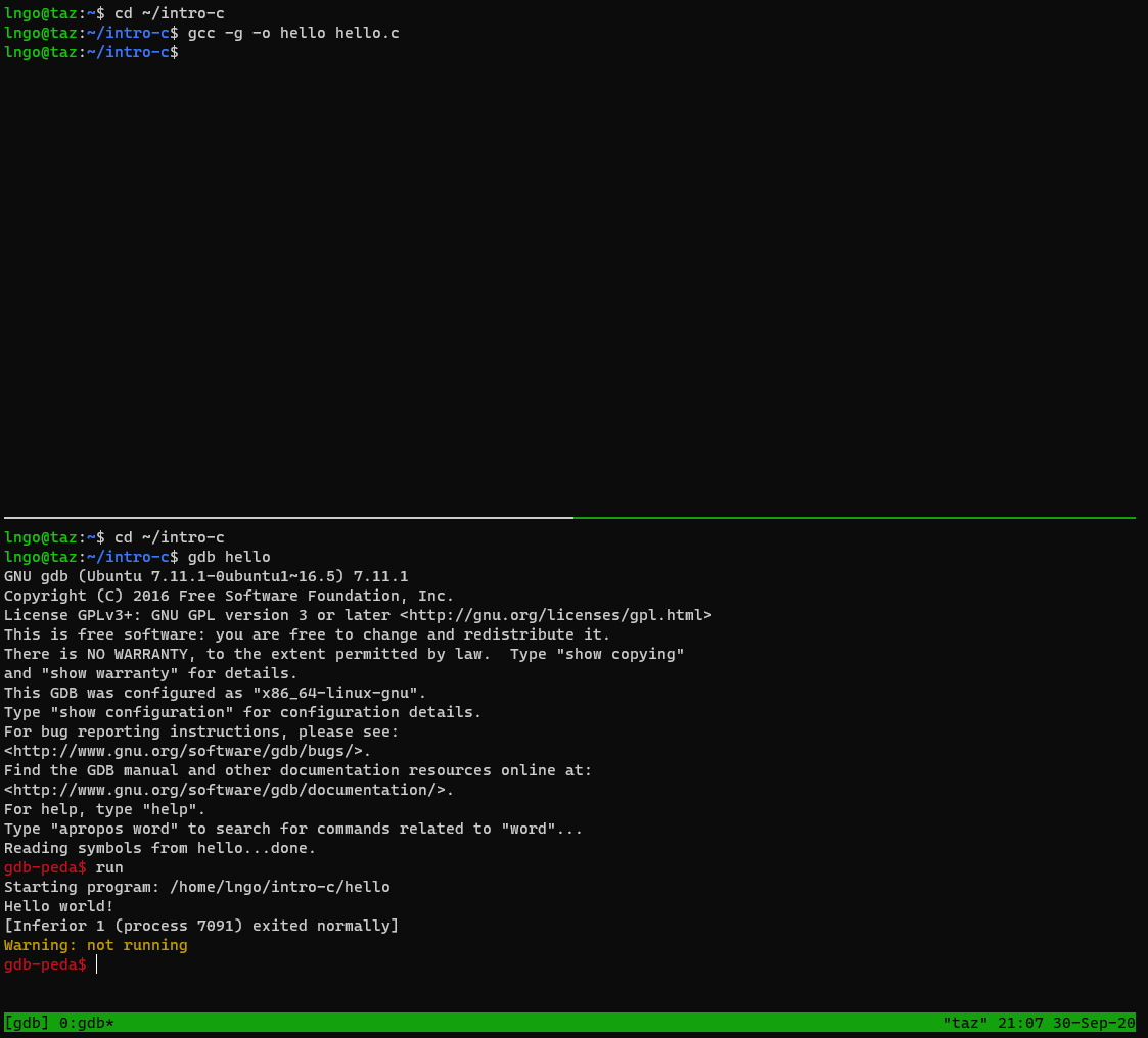
To use gdb to debug, we need to compile the program with a -g flag.

Split the gdb session into two horizontal panes.

In the top pane, run the followings command:
$ cd ~/csc331/intro-c
$ gcc -g -o hello hello.c
In the bottom pane, run the followings command:
$ cd ~/csc331/intro-c
$ gdb hello
gdb-peda$ run

13. Debugging with gdb

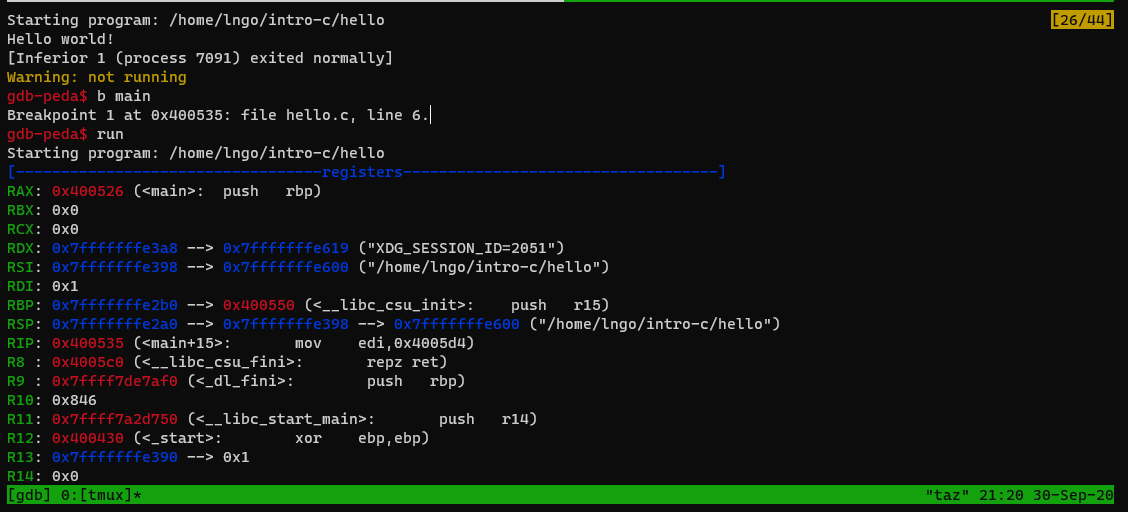
We need to set a breakpoint:

Could be a line number or

Could be a function name
gdb-peda$ b main
gdb-peda$ run

15. Scrolling within tmux’s panes

Mouse scrolling does not work with tmux.

To enable scrolling mode in tmux, type Ctr-b then [.

You can use the Up/Down/PgUp/PgDn keys to navigate.

To quit scrolling mode, type q or Esc.
gdb-peda$ b main
gdb-peda$ run
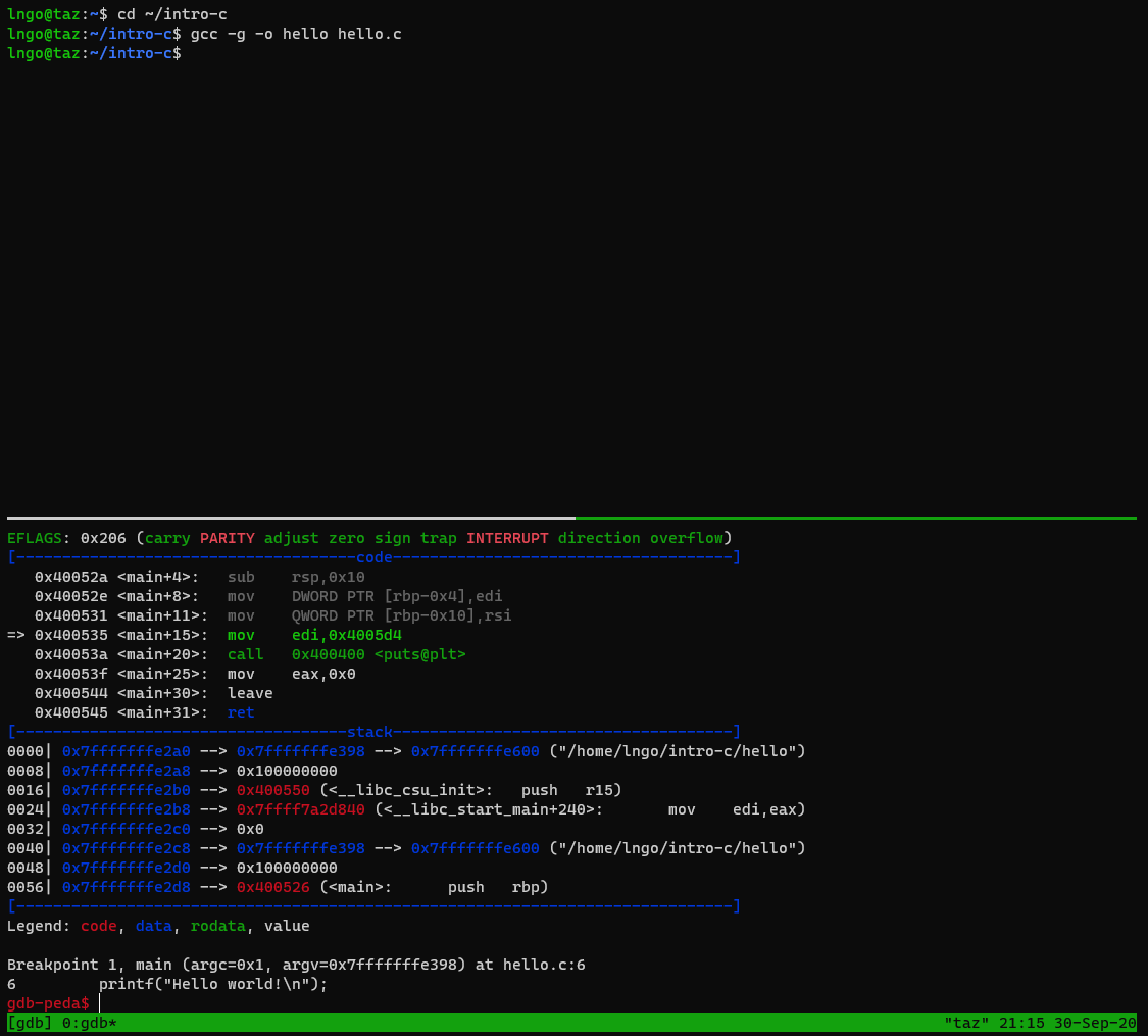
At a glance

Registers’ contents

Code

Stack contents

Assembly codes

gdb stops at our breakpoint, just before function main.

The last line (before the gdb-peda$ prompt) indicates the next line of code to be executed.

16. Hands on: finish running hello

Type q or Esc to quit scrolling mode.

To continue executing the next line of code, type n then Enter.

Turn back into the scrolling mode and scroll back up to observe what happens after typing n.

What is the next line of code to be executed?

Type n three more times to observe the line of codes being executed and the final warning from gdb.

17. Examining contents of program while debugging
In the top pane, compile malloc_1.c in debugging mode.

In the bottom pane, quit the current gdb session and rerun it on the recently created malloc_1 executable.
Setup main as the breakpoint and start running.
gdb-peda$ b main
gdb-peda$ run
Type n and Enter to run the next line of code: void *p = malloc(4);

Type p p: the first p is short for print and the second p is the void pointer variable p in the program.

Try running p *p. What does that feedback mean?

Type n and Enter to run the next line of code: float *fp = (float *)p;

Type p fp: what is the printed value?

Type n and Enter to run the next line of code: int *ip = (int *)p;

Type p ip: what is the printed value?

Type n and Enter to run the next line of code: *ip = 98765;

Type p ip: what is the printed value?

Type p *ip: what is the printed value?

Type p /t *ip: what type of data is value? what is the corresponding value in decimal?

Keep hitting n until you finish stepping through all the remain lines of code.

18. Examining contents of program while debugging

In the top pane, compile array_4.c in debugging mode.

In the bottom pane, quit the current gdb session and rerun it on the recently created array_4 executable as follows:
$ gdb array_4
gdb-peda$ b main
gdb-peda$ run
The next line of code to be run is size = atoi(argv[1]);

Run the following commands and observe the outcomes:

p argc

p argv[0]

p argv[1]

p argv[2]

p argv[3]

p argv[4]

…

Type n and Enter to run the next line of code: size = atoi(argv[1]);

Turn into scrolling mode to observe that dreaded Segmentation fault notice.

Scrolling down to see if gdb helps identify the issue?

Type q to exit gdb.

Rerun gdb on array_4 executable as follows:
$ gdb array_4
gdb-peda$ b main
gdb-peda$ run 3
The next line of code to be run is size = atoi(argv[1]);

Run the following commands and observe the outcomes:

p argc

p argv[0]

p argv[1]

p argv[2]

…

Type n and Enter to run the next line of code: size = atoi(argv[1]);

Run the following commands and observe the outcomes:

p size

p &size

Type n and Enter to run the next line of code: printf("Before malloc, p is pointing to address (%p)\n", p);

Run the following commands and observe the outcomes: p p

19. Hands on: finish running array_4

Step through the for loop and printing out values of i, p[i], &p[i], and p + i at every iteration.

Make sure that you understand the lines of code that cause these variables to change value.

Utilize scrolling as needed.

Key Points

First key point. Brief Answer to questions. (FIXME)

Memory virtualization

Overview

Teaching: 0 min
Exercises: 0 min

Questions

How can an illusion of infinite and isolated memory space be managed?

Objectives

Understand how a process’ components are organized in memory.

Understand the idea of address space and memory virtualization.

0. Midterm Exam…

Wednesday, March 24 , 2021

24-hour windows range: 12:00AM - 11:59PM March 24, 2021.

75 minutes duration.

20 questions (similar in format to the quizzes).

Everything (including source codes) up to today (Wednesday, March 3, 2021).

1. In the beginning …

Users didn’t expect much.

To be honest, most, if not all, users are also developers …

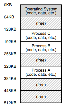
2. Early systems

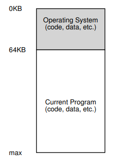
Computers run one job at a time.

The OS was preloaded into memory and consisted of a set of routines.

There was one running program that uses the rest of memory.

3. Multiprogramming and time sharing

Demands for

Utilization

Efficiency

Interactivity

Multiple processes ready to run at a given time.

The OS switches between them.

One approach is to run one process at a time and still give it full access to all memory (just like the early days …).

This requires switch processes from memory.

4. Multiprogramming and time sharing

This solution does not scale as memory grows.

System event Size Latency

CPU <1ns

L1 cache 32KB 1ns

L2 cache 256KB 4ns

L3 cache >8MB 40ns

DDR RAM 4GB-1TB 80ns

System event	Size	Latency
CPU		<1ns
L1 cache	32KB	1ns
L2 cache	256KB	4ns
L3 cache	>8MB	40ns
DDR RAM	4GB-1TB	80ns

5. Multiprogramming and time sharing

What we want to do

Leave processes in memory and let OS implement an efficient time sharing/switching mechanism.

A new demand: protection (through isolation)

6. Address space

Provide users (programmers) with an easy-to-use abstarction of physical memory.

The running program’s view of memory in the system.

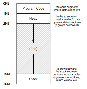
Contains all memory states of the running program:

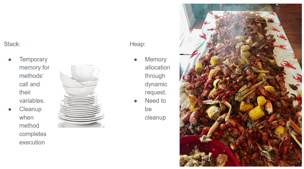
Stack to keep track of where it is in the function call chain (stack frames), allocate local variables, and pass parameters and return values to and from routines.

Heap is used for dynamically allocated, user-managed memory (i.g., malloc()).

BSS (block started by symbols) contains all global variables and static variables that are initialized to zero or do not have explicit initialization in source code.

Data contains the global variables and static variables that are initialized by the programmer.

Code (binary) of the program.

One visual representation of address space

Another visual representation of address space

Image taken from Geeksforgeeks

7. Hands on: what is in your binary?

Open a terminal (Windows Terminal or Mac Terminal).

Run the command to launch the image container for your platform:

Windows:
$ podman run --rm --userns keep-id --cap-add=SYS_PTRACE --security-opt seccomp=unconfined -it -v /mnt/c/csc331:/home/$USER/csc331:Z localhost/csc-container /bin/bash
Mac:
$ docker run --rm --userns=host --cap-add=SYS_PTRACE --security-opt seccomp=unconfined -it -v /Users/$USER/csc331:/home/$USER/csc331:Z csc-container /bin/bash
Navigate to /home/$USER/csc331

Change to directory ostep-code/cpu-api, then run make to build the programs.

Launch a tmux session called m1 with two vertical panels.

In the left panel, run the following commands:
$ mkdir ~/memory 
$ cd ~/memory 
Create a C program named simple.c inside directory memory.

Reminder: The sequence to create/edit files using nano is as follows:

Run nano -c ile_name

Type in the contents

When done, press Ctrl-X

Press y to confirm that you want to save modification

Press Enter to confirm the file name to save to.

Create simple.c with the following contents:

In the left panel, run the followings:
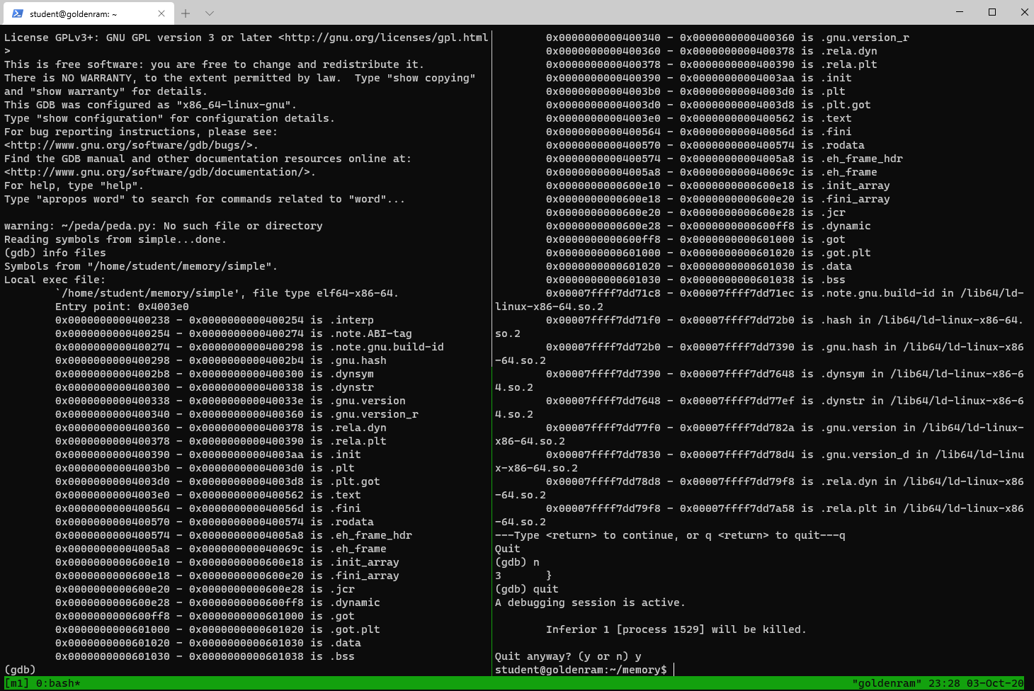
$ gcc -g -o simple simple.c 
$ gdb simple 
gdb-peda$ info files
In the right panel, run the followings:
$ cd ~/memory 
$ gdb simple
gdb-peda$ b main
gdb-peda$ run
gdb-peda$ info files
The left panel shows the binary file, which is basically a packing list.

The right panel shows how the contents are loaded from static libraries (with memory changed)

Move to the right panel and press Enter to continue going through the list.

Go through the remaining steps (using n) of the debugging process until finish.

Quit gdb instances in both panels.

8. Hands on: what is in your binary?

Disable address randomization (permanently).

You only need to do this once using either tmux panels.
$ echo 0 | sudo tee /proc/sys/kernel/randomize_va_space
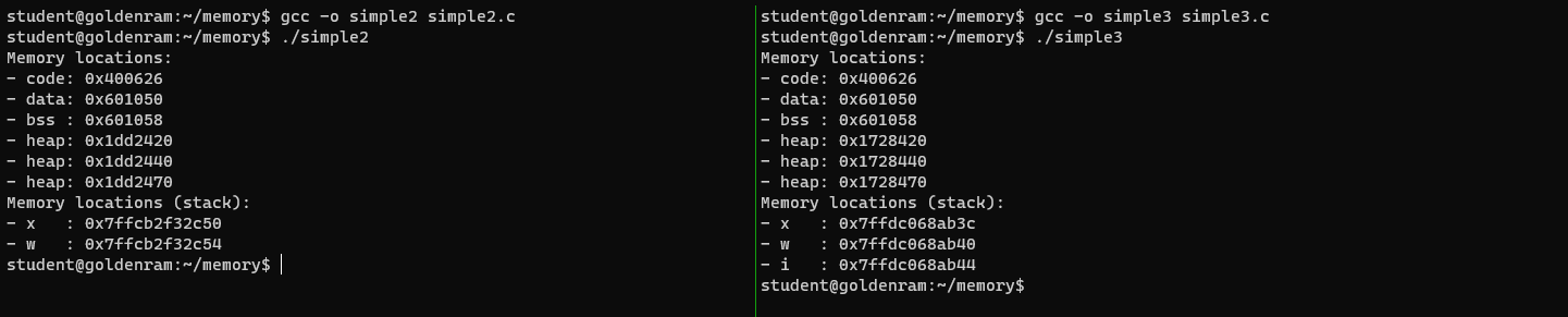
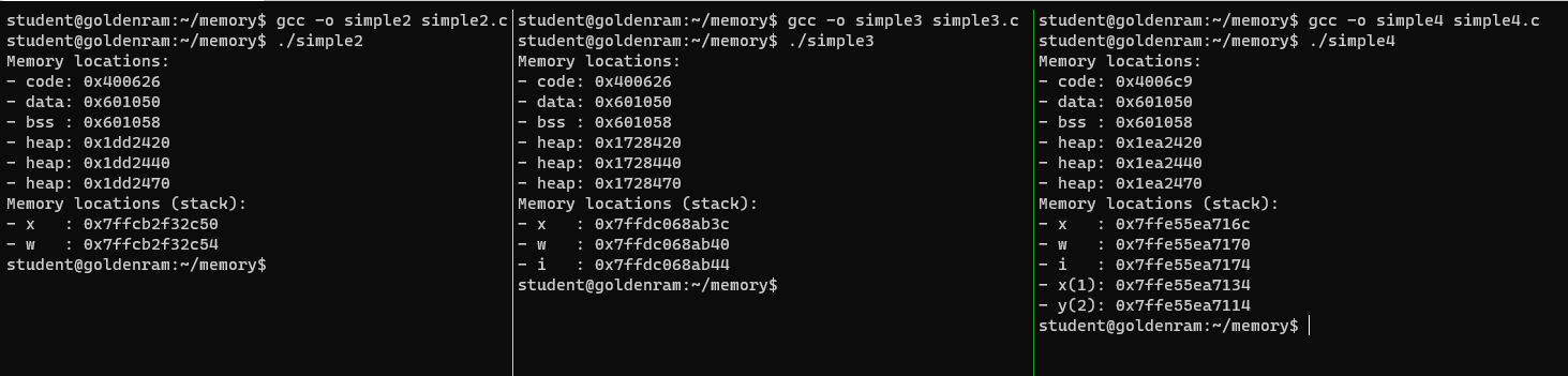
In the left panel, create simple2.c inside memory with the following contents:

In the right panel, create simple3.c inside memory with the following contents:

Compile and run simple2.c and simple3.c normally.

Compare the output.

But Dr. Ngo just said the stack grows downward …?

9. Hands on: where the stack grows?

Add one more vertical panel to your tmux session.

Adjust the panels’ width (resize-pane -L/-R) so that they balance.

In the new panel, create simple4.c inside memory with the following contents:

Stack grows downward (high to low) relative to stack frames …

Within a stack frame, memory reserved for data are allocated in order of declaration from low to high

10. Hands on: observing inner growth (of the stacks)?

In the first or second panel (the one next to the result from running simple4, create a copy of simple4.c called simple5.c.

Modify simple5.c to print out one or two additional variables in each of the functions f1 and f2.

Compile and run simple5.c to observe how within each stack frame, memory are allocated in the order from low to high.

In the new panel, create simple4.c inside memory with the following contents:

11. What is address space, really?

The abstraction of physical memory that the OS is providing to the running program.

How can the OS build this abstraction of a private, potentially large address space for multiple running processes on top of a single physical memory?

This is called memory virtualization.

12. Goals of memory virtualization

Transparency: The program should not be aware that memory is virtualized (did you feel anything different when programming?). The program should perceive the memory space as its own private physical memory.

Efficiency: The virtualization process should be as efficient as possible

Time: not making processes run more slowly

Space: not using too much memory for supporting data structures

Protection: Protection enable the property of isolation: each process should be running in its own isolated memory space, safe against other processes.

13. Dr. Ngo loves his analogies

In the firgure to the right, what represents the heap?

14. Hands on: is memory unlimited?

Reduce the number of vertical panels down to 2 and adjust the sizes (see screenshot below).

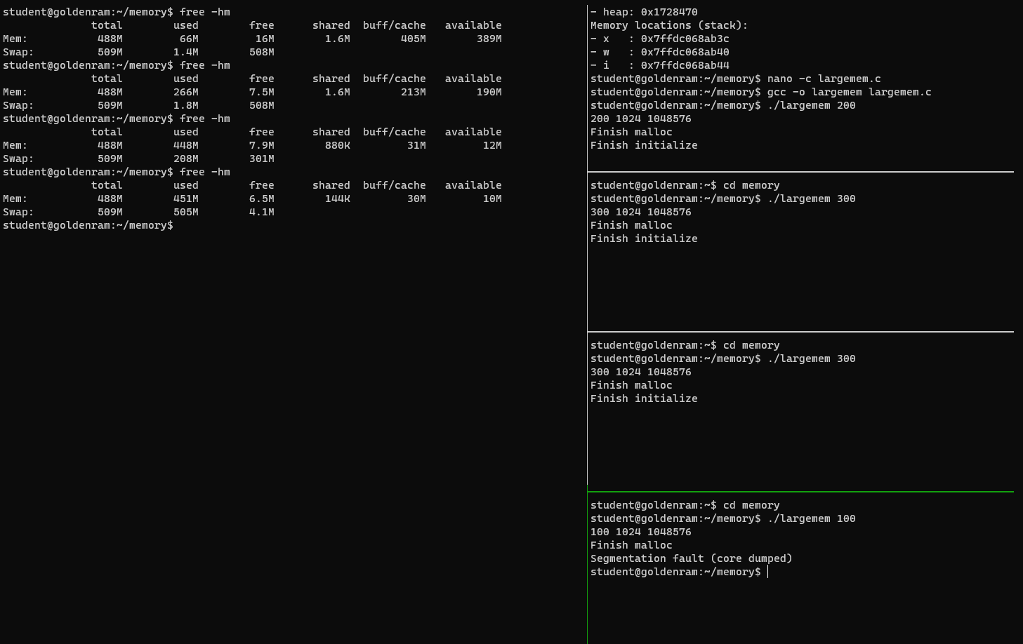
In one of the panels, create largemem.c inside memory with the following contents, then compile.

Split the right vertical panel to four (or more) horizontal panels.

In the left panel, first run free -hm and study the output.

In the top right panel, inside memory, run largemem with a command line argument of 200.

In the left panel, rerun free -hm and study the new output.

Subsequently, alternatve between running largemem in the right panels and free -hm in the left panel, adjusting the command line argument of largemem such that you run into a segmentation fault in the last panel.

This is the impact of memory allocation (reservation).

Key Points

Memory virtualization is how the OS provides an abstraction of physical memory to process in order to facilitate transparency, efficiency, and protection.

Memory virtualization mechanism: address translation

Overview

Teaching: 0 min
Exercises: 0 min

Questions

How to efficiently and flexibly virtualize memory

Objectives

Understand the design principles behind an efficient memory virtualization implementation.

Understand the required flexibility for applications.

Understand how to maintain control over memory location accessibility.

1. The questions?

How can we build an efficient virtualization of memory?

How do we provide the flexibility needed by applications?

How do we maintain control over which memory locations an application can access?

2. General technique

Hardware-based address translation (address translation)

HW transforms virtual address from memory access into physical address.

The OS gets involved to ensure correct translations take place and manage memory to keep track of and maintain control over free and used memory locations.

3. Initial assumptions

User’s address space must be place contiguously in physical memory.

The size of the address space is less than the size of physical memory.

Each address space is exactly the same size.

4. Hands on: revisiting where things are in memory

Open a terminal (Windows Terminal or Mac Terminal).

Run the command to launch the image container for your platform:

Windows:
$ podman run --rm --userns keep-id --cap-add=SYS_PTRACE --security-opt seccomp=unconfined -it -v /mnt/c/csc331:/home/$USER/csc331:Z localhost/csc-container /bin/bash
Mac:
$ docker run --rm --userns=host --cap-add=SYS_PTRACE --security-opt seccomp=unconfined -it -v /Users/$USER/csc331:/home/$USER/csc331:Z csc-container /bin/bash
Navigate to /home/$USER/csc331

Change into memory directory.

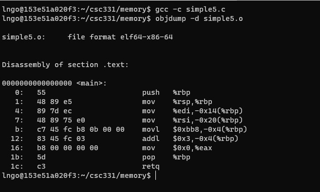
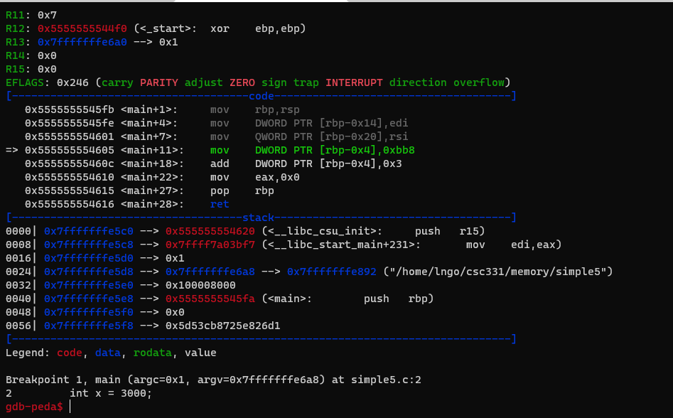
Create a file named simple5.c with the following contents:

Compile and view simple5.c object file
$ gcc -c simple5.c
$ objdump -d simple5.o
What is the decimal value of 0xbb8?

Compile with -g for simple5.c.

Execute gdb simple5, set breakpoint at main, and start running.

Where is the variable x is? (run p &x to find out)

What is the difference between the value contained in %ebp and the address of x?

Where is the machine instruction? (code)

Where are their location in address space?

5. Initial assumptions

User’s address space must be place contiguously in physical memory.

The size of the address space is less than the size of physical memory.

Each address space is exactly the same size.

6. Early attempt: dynamic relocation

Hardware-based

Aka base and bounds

Two hw registers within each CPU:

Base register

Bounds (Limit) register
physical address = virtual address + base
0 <= virtual address <= bound

7. Dynamic relocation: after boot

8. Dynamic relocation: during process run

9. Dynamic relocation: Summary

Pros:

Highly efficient through simple translation mechanisms

Provides protection

Cons:

Wastage through internal fragmentation due to space inside the allocated (contiguous) memory units are not fully utilized.

10. Initial assumptions

~~~User’s address space must be place contiguously in physical memory.~~~

~~~The size of the address space is less than the size of physical memory.~~~

~~~Each address space is exactly the same size.~~~

How do we support a large address space with (potentially) a lot of free space between the stack and the heap?

11. Segmentation: generalized base/bounds

Original: One base/bound pair for one address space.

Segmentation: One base/bound pair per logical segment of an address space:

Code

Stack

Heap

12. Segmentation: generalized base/bounds

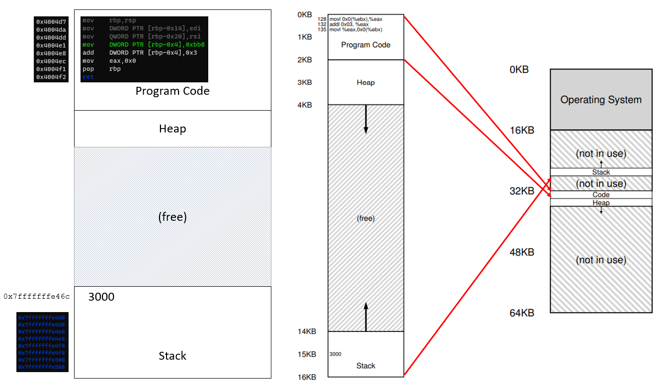
13. Example

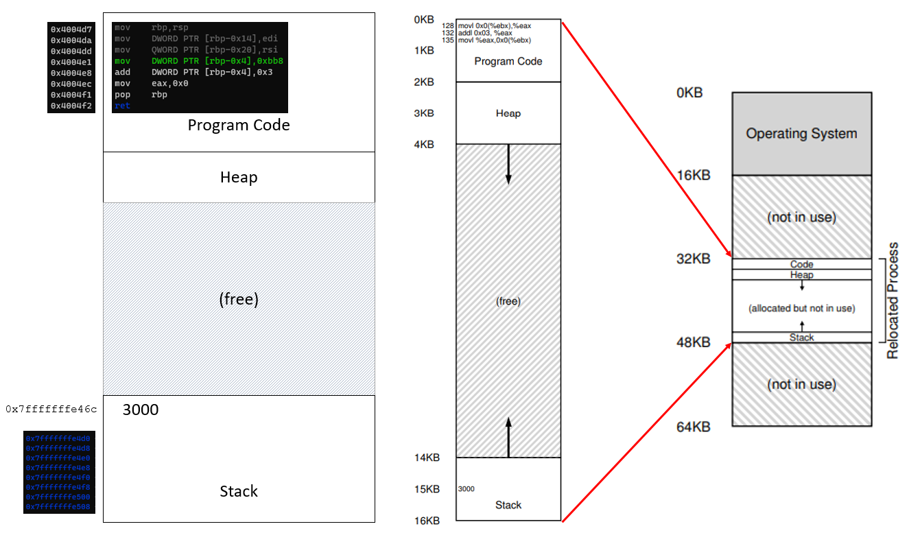
Note: 32K = 2¹⁵ = 32768

Segment Virtual segment base Virtual segment bound Physical segment base Physical segment bound Size

Code 0KB 2KB 32KB 34KB 2KB

Heap 4KB 6KB (can grow up) 34KB 36KB 2KB

Stack 16KB 14KB (can grow down) 28KB 26KB 2KB

Reference is made to virtual address 100 (code segment)

This is called the offset

physical address = physical segment base + offset = 32K (32768) + 100 = 32868

Reference is made to virtual address 4200 (heap segment)

What is the correct offset:

offset = virtual address - virtual segment base = 4200 - 4096 = 104

physical address = physical segment base + offset = 34K (34816) + 104 = 34920

Reference is made to virtual address 7000?

Look likes heap segment

Is it heap segment?

offset = virtual address - virtual segment base = 4200 - 4096 = 2904

physical address = physical segment base + offset = 34K (34816) + 2904 = 37720

This falls into physical addresses that are markedas not in use.

Segmentation Fault: AKA segmentation violation

Illegal virtual address

Segment	Virtual segment base	Virtual segment bound	Physical segment base	Physical segment bound	Size
Code	0KB	2KB	32KB	34KB	2KB
Heap	4KB	6KB (can grow up)	34KB	36KB	2KB
Stack	16KB	14KB (can grow down)	28KB	26KB	2KB

14. Segmentation with generalized base/bounds: Summary

Pros:

Efficient saving of physical memory (avoid internal fragmentation)

Enable the creation of segments with various sizes

Cons:

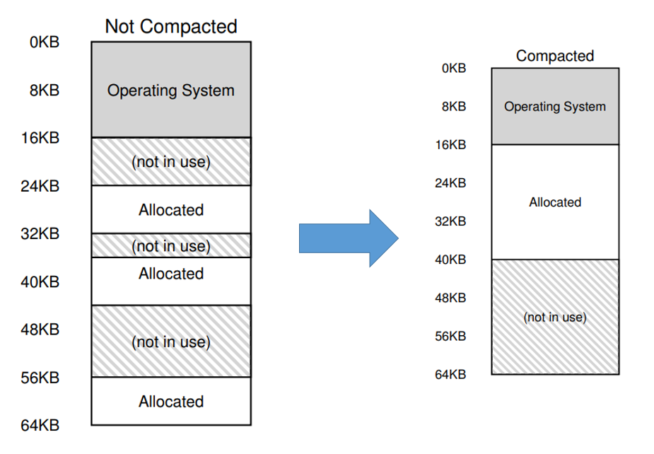
External fragmentation

15. External fragmentation: compacting

Computationally expensive

16. External fragmentation: algorithmic allocation

A data structure that keeps track of free memory regions:

Best-fit

Worst-fit

First-fit

Next-fit

Buddy algorithm

Does not address the core of the issue, only minimize it as much as possible. New solution is needed!

Key Points

First key point. Brief Answer to questions. (FIXME)

Memory virtualization mechanism: paging and tlb

Overview

Teaching: 0 min
Exercises: 0 min

Questions

How to virtualize memory with pages to minimize segmentation issues?

How to speed up address translation?

Objectives

Understand the overall concept of paging.

Understand the data structure for page tables.

1. What is paging?

Divide contents into fixed-size units, called pages.

Each page has a page number

Locate contents in pages by an offset (10th word on page 185)

There is a table to tell you which content is on which page

Physical memory is viewed as an array of fixed-size slots called page frames.

Each frame can contain a single virtual memory page

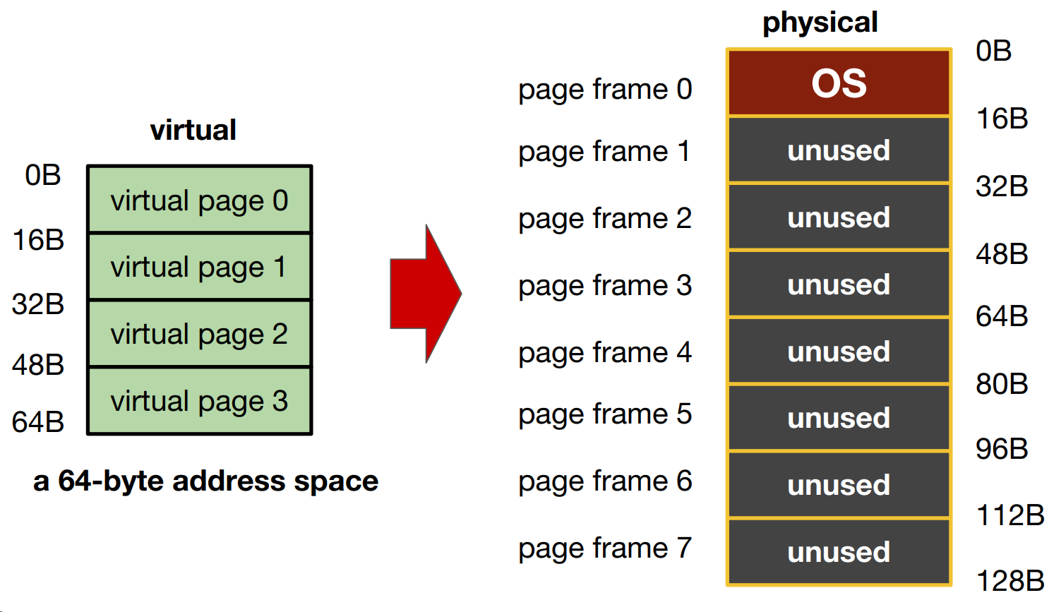
2. After allocation

For allocation management, the OS keeps a list of free (fixed-size) pages.

This is much simpler than trying to maintain a list of variable-size memory regions

Virtual pages are numbered, which preserve the order of the virtual address space. This allows us to allocate page frame for the virtual pages across the entire available physical memory space.

3. What data structure is needed?

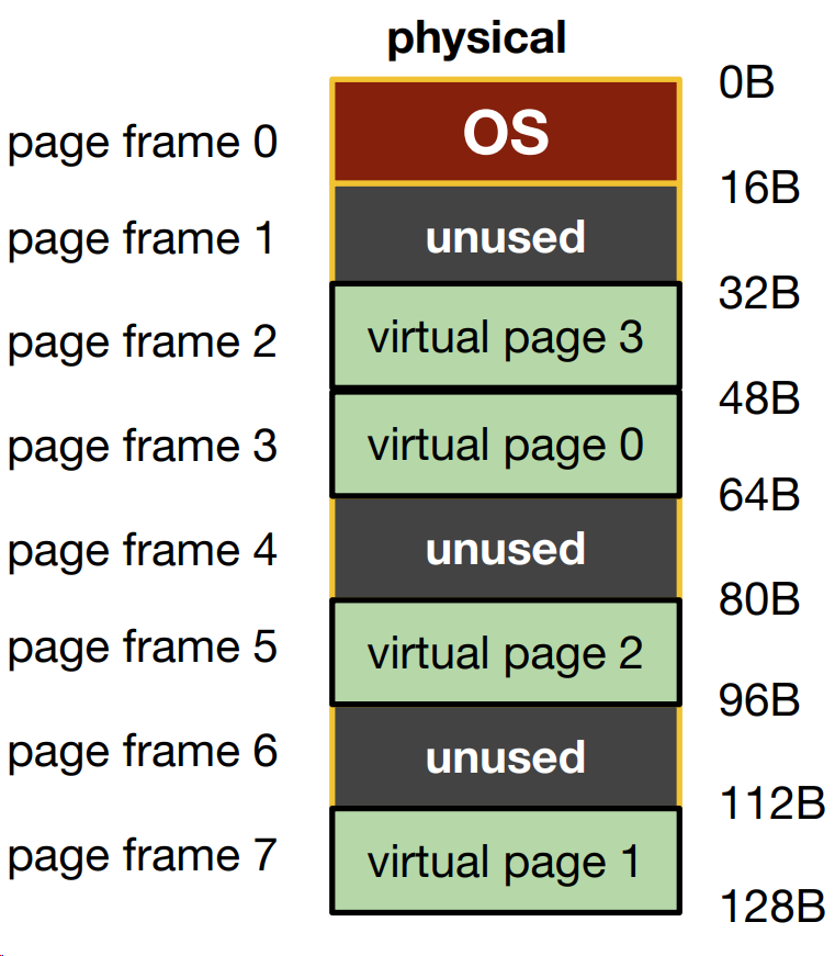
Page Table: Mapping from virtual page number to physical page frame

VP0 -> PF3

VP1 -> PF7

VP2 -> PF5

VP3 -> PF2

Each process has its own page table

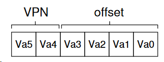
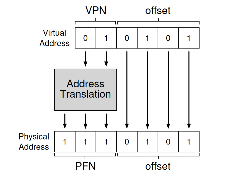
4. Address translation with paging.

To translate a virtual address, we need:

Virtual page number (VPN)

The offset within the page

For the 64-bit virtual address space, 6 bytes are needed (2⁶ = 64)

There are four pages (2 bytes for VPN)

Each page stores 16 bytes (4 bytes to describe offset of these 16 bytes).

The physical memory has 128 bit, so the physical address will be 7 bytes.

The 2-byte VPN (virtual page number) will be translated to a corresponding 3-byte PFN (page frame number).

The offset remains the same (virtual page has the same size as page frame).

5. New questions!

What are the typical contents of the page table?

How big are the page tables?

Where are the page tables stored?

Does paging slow down the system?

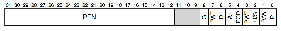
6. Contents of a page table entry (PTE) for 32-bit x86

PFN: 20 bits for physical page frame number (page size 4K)

P: present bit, whether this page is on memory or on disk (swapped)

R/W: read/write bit, whether writes are allowed to this page

U/S: user/supervisor bit, whether user-mode processes can access this page

A: access bit, whether this page has been accessed

D: dirty bit, whether this page has been modified

PWT, PCD, PAT, G: how hardware caching works for this page

7. Size of page table 32-bit x86

Typical page size is 4KB (run getconf PAGESIZE in your VM to observe this)

Size of address space: 4GB

Number of pages in address space: 4GB / 4KB = 1M

Number of PTE in page table: 1M

How many bits for VPN: 20

How many bits for offset: 12

Each PTE is 4 bytes, therefore the size of a page table is 4B * 1M = 4MB per process

Assume 100 processes running, we have 400MB of all page tables

This is too big

8. How can we reduce the size of the page table?

Bigger pages.

Hybrid: Page + Base/Bound

Multi-level page tables

9. Bigger pages

Let the page size be 16K instead of 4K

4GB address space

Number of pages in address space: 4GB / 16KB = 256K

Number of PTE in page table: 256K

How many bits for VPN: 18

How many bits for offset: 14

Each PTE is 4 bytes in size

Total size of page table is 256K * 4B= 1M

Smaller by a factor of 4

Problem:

For small processes, we waste the remaining space of a page.

This is internal fragmentation

10. Hybrid

Separate page tables for stack, heap, and code.

For each page table, use base/bound register to keep the physical address of the page table.

Use two bits in the virtual address to indicate which segment it is in.

No need to have PTEs for unused paged.

Problem: Bring back all issues of segmentation

Free space management

External fragmentation

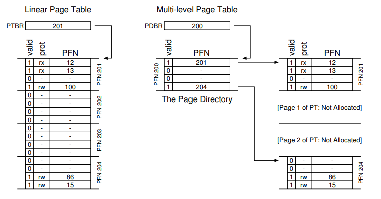
11. Multi-level page tables

Overall idea

Chop up the page table into page-sized units.

If an entire page of page-table entries is invalid, don’t allocate that page of the page table at all (reduce memory space).

A new structure called page directory is needed to keep track of pages’ validity

12. Multi-level page tables

Two-level table

One entry per page of page table (Page Directory Entry - PDE)

A PDE has a valid bit and a page frame number (PFN)

If the PDE is valid, it means that at least one of the the pages of the page table that the entry points to (via the PFN) is valid.

If the PDE is not valid, the rest of the PDE is not defined.

13. Multi-level page tables: advantages

Only allocates page-table space in proportion to the amount of address spaces being used.

If carefully constructed, each portion of the page table fits neatly within the page, making it easier to manage memory (think pointer to memory space versus contiguous memory location).

14. Multi-level page tables: cost

Space versus Time: To reduce space, increased access translation steps are needed: one for the page directory and one for the PTE itself.

Complexity: Page table lookup is more complex to implement than a simple linear page-table look up.

15. Multi-level page tables: cost

Each level of multi-level page tables requires one additional memory access:

One to get PTE.

One to get the actual data.

Linux can go up to 4 level of page tables

Hardware to the rescue!

Translation Lookaside Buffer (aka TLB, aka address translation cache, aka cache)

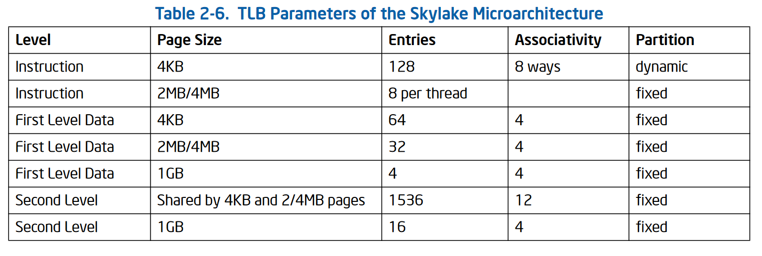
16. Translation Lookaside Buffer

Part of the memory management unit (MMU)

Small, fully associative hardware cache of recently used translations

small, so it’s fast by laws of physics

fully associative, i.e., all entries looked up in parallel, so it’s fast

hardware, so it’s fast

It is so fast that the lookup can be done in a single CPU cycle.

A successful lookup in TLB is called a TLB hit, otherwise it is a TLB miss

17. What is in TLB?

Lookup entries: VPN -> PFN plus some other bits

A TLB typically has 32, 64, or 128 entries

18. First issue with TLB

Context switch invalidates all entries in TLB. Why?

Because the VPN stored in a TLB entry is for current process, which becomes meaningless when switched to another process.

Could lead to wrong translation if not careful.

Possible solutions:

Simply flush the the TLB on context switch, i.e., set all valid bits to 0.

Safe, but inefficient.

Think of two Processes A and B that frequently context switch between each other.

Add Address Space Identifier (ASID) to TLB entry

It’s basically PID, but shorter (e.g., 8 bits instead of 32 bits)

Avoids wrong translation without having to flush all entries

19. Second issue with TLB

Replacement policy

When TLB is full, and we want to add a new entry to it, we will have to evict an existing entry.

Which one to evict?

20. TLB and locality

Processes only use a handful of pages at a time.

A TLB with 64 entries can map 64 * 4K = 192KB of memory, which usually. covers most of the frequently accessed memory by a process within certain time span.

In reality, TLB hit rates (hit / (hit + miss)) are typically very high (> 99%).

Caching is an important idea, use it when possible.

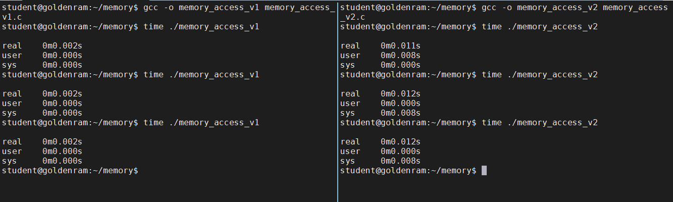
21. Hands on: memory access

Open a terminal (Windows Terminal or Mac Terminal).

Run the command to launch the image container for your platform:

Windows:
$ podman run --rm --userns keep-id --cap-add=SYS_PTRACE --security-opt seccomp=unconfined -it -v /mnt/c/csc331:/home/$USER/csc331:Z localhost/csc-container /bin/bash
Mac:
$ docker run --rm --userns=host --cap-add=SYS_PTRACE --security-opt seccomp=unconfined -it -v /Users/$USER/csc331:/home/$USER/csc331:Z csc-container /bin/bash
Launch a tmux session called mem with two vertical panels.

Create two vertical panels.

In the left panel, change to directory memory and create memory_access_v1.c with the following contents:

In the right panel, change to directory memory and create memory_access_v2.c with the following contents:

Questions

Which is faster?

Why?

In the left panel, compile and timed run memory_access_v1.c:
$ gcc -o memory_access_v1 memory_access_v1.c
$ time ./memory_access_v1
In the right panel, compile and timed run memory_access_v2.c.
$ gcc -o memory_access_v2 memory_access_v2.c
$ time ./memory_access_v2

22. Demand paging

In an ideal world, we have an infinite amount of RAM …

In reality:

Many processes use memory, and in combination exceeds the size of physical memory.

One process’ memory usage can be larger the size of physical memory.

OS supports a mechanism to offload exceed memory demands to hard disks to store pages that are not being accessed.

From the perspective of processes, everything is still within a large virtual address space.

This mechanism is called demand paging.

23. Demand paging

Swap space: a reserved space on hard disk for moving pages back and forth

Linux/Unix: a separate disk partition

Windows: a binary file called pagefile.sys

Initially, pages are allocated in physical memory.

As memory fills up, more allocations require existing pages to be evicted.

Evicted pages go to disk (into swap space).

24. Demand paging

Present bit (P) indicates whether the page is in memory or on disk.

P = 0 (on disk), then the remaining bits in PTE store the disk address of the page.

When the page is loaded into memory, P is set to 1, and the appropriate PTE contents are updated.

25. Demand paging control flow

If the page is in memory, keep going.

If the page is to be evicted, the OS sets P to 0, moves the page to swap space, and stores the location of the page in the swap space in the PTE.

When a process access the page, the 0 value of P will cause a system trap called page fault.

The trap run the OS page_fault_handler, which locates the page in the swap file.

The trap reads the page into a physical frame, and updates PTE to points to this frame.

The trap returns to the process, and the page will be available for the process.

26. Dirty bit

If the page has been not been modified (dirty == 0) since it was loaded from swap, nothing will need to be written to disk when the page is evicted again.

If the page has been modified (dirty == 1), it must be rewritten to disk when it is evicted.

This mechanism is invented by Corbato. (Who is Corbato?).

Issue:

When we have to evict a page to disk, which one should we choose?

27. Replacement algorithms

Reduce fault/miss rate by selecting the best victim to evict.

Unrealistic assumption: we know the whole memory reference trace of the program, including the future ones at any point in time.

Algorithm 1: evict the one that will never be used again.

Does not always work.

Algorithm 2: evict the page whose next access is furthest in the future.

Belady’s algorithm (“A study of replacement algorithm for a virtual-storage computer”, IBM Systems Journal, 5(2), 1966).

Caveat: we don’t know the future.

Belady’s algorithm serves as the benchmark to see how close other algorithms are to being perfect!

28. We predict the future based on patterns …

Locality: the patterns in computer programs’ behaviors.

Spatial locality: If an address A is accessed, then addresses A - 1 and A + 1 are also likely to be accessed.

Temporal locality: if an address is accessed at time T, then it is also likely to be accessed again in the future T + Δt.

This is not a set-in-stone rule, but in general, it is a good heuristic to remember when designing computing systems.

29. Example policies

FIFO:

Good: oldest page is unlikely to be used again.

Bad: oldest page is likely to be used again.

Random:

Based purely on luck.

TLB replacement is usually random.

LRU:

Least recently used.

Close to optimal.

Not very easy to implement.

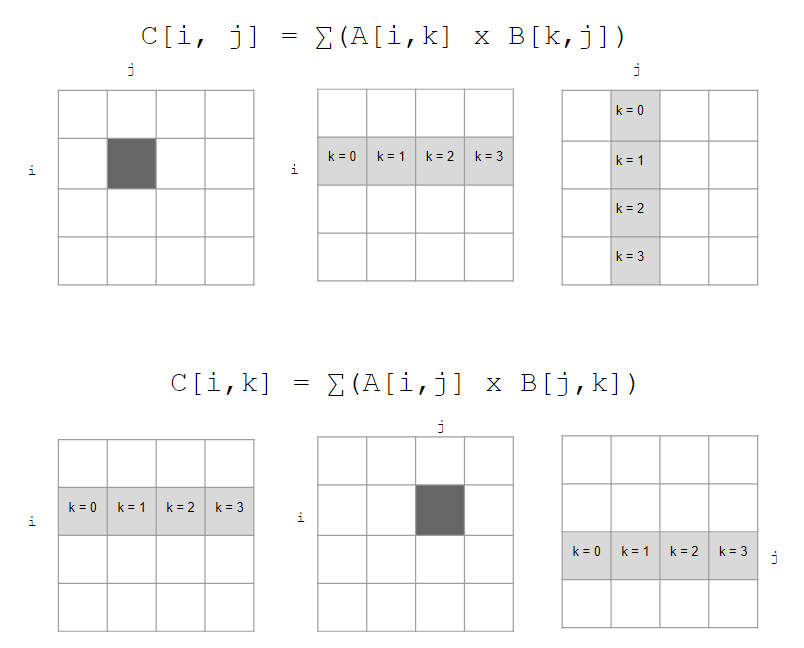
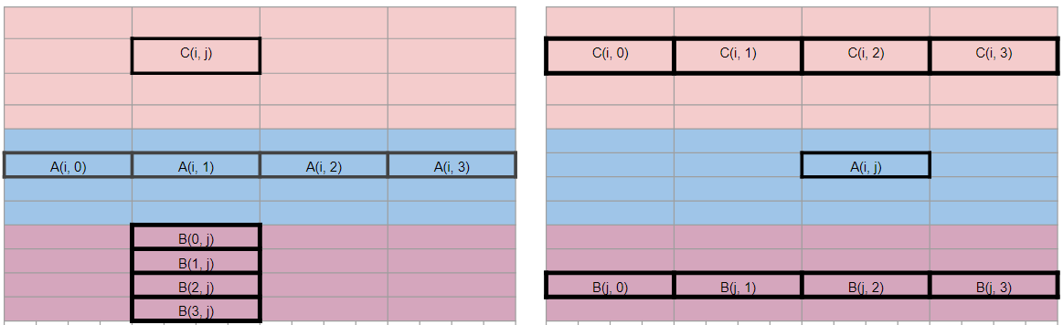
30. Matrix multiplication

Which approach is faster?

Why?

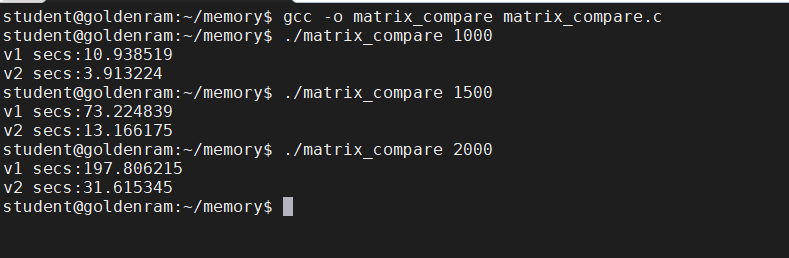
31. Hands on: matrix multiplication

In the left panel, change to directory memory and create matrix_compare.c with the following contents:

Questions

Which matrix multiplication function (matrix_mul_v1 or matrix_mul_v2) represents which multiplication approach from slide 30?

Compile and run matrix_compare.c:
$ gcc -o matrix_compare matrix_compare.c
$ ./matrix_compare 1000
$ ./matrix_compare 1500
$ ./matrix_compare 2000

Key Points

First key point. Brief Answer to questions. (FIXME)

Introduction to concurrency using threads

Overview

Teaching: 0 min
Exercises: 0 min

Questions

How to support concurrency?

Objectives

First learning objective. (FIXME)

1. Review: process calls fork()

New PCB (process control block) and address space.

New address space is a copy of the entire contents of the parent’s address space (up to fork).

Resources (file pointers) that point to parent’s resources.

In general, time consuming.

2. Review: process context switch

Save A’s registers to A’s kernel stack.

Save A’s registers to A’s PCB.

Restore B’s registers from B’s PCB.

Switch to B’s kernel stack.

Restore B’s registers from B’s kernel stack.

In general, time consuming.

3. Example: web server

A process listens to requests.

When a new request comes in, a child process is created to handle this request.

Multiple requests can be handled at the same time by different child processes.

What is the problem?
while (1) {
	  int sock = accept();
  if (0 == fork()) {
    handle_request();
    close(sock);
    exit(0);
  }
}

4. Thread: a new abstraction for running processes

A normal process is a running program with a single point of execution, i.e, a single PC (program counter).

A multi-threaded program has multiple points of execution, i.e., multiple PCs.

Each thread is very much like a separate process, except for one difference:

All threads of the same process share the same address space and thus can access the same data.

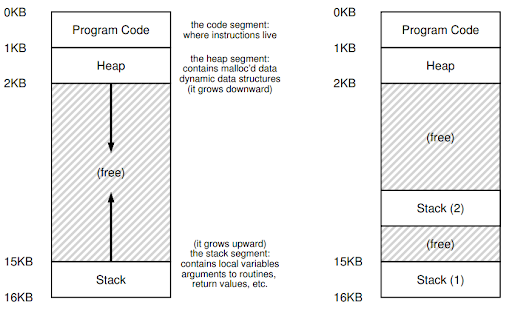
5. Thread: state of a single thread

Each thread has its own PC.

Each thread has its own private set of registers for computation.

Context switching is still needed.

Threads use Thread Control Blocks (TCP) to store their execution states.

Context switching is similar to that of processes, except for:

Thread context-switching keep the same address space (i.e., no need to switch out the page table).

6. Example: web server using thread

int global_counter = 0;
web_server() {
  while (1) {
    int sock = accept();
    thread_create(handle_request, sock);
  }
}

handle_request(int sock) {
  process request;
  ++global_counter;
  close(sock);
}

7. API: POSIX threads (pthreads)

Standardized C language thread programming API.

pthreads specifies the interface of using threads, but not how threads are implemented in OS.

Different implementations include:

kernel-level threads,

user-level threads, or

hybrid

pthread_create

pthread_join

8. Hands on: say hello to my little threads …

Before turning on the VM, makes sure that you have two processors assigned to your VM.

Open a terminal (Windows Terminal or Mac Terminal).

Run the command to launch the image container for your platform:

Windows:
$ podman run --rm --userns keep-id --cap-add=SYS_PTRACE --security-opt seccomp=unconfined -it -v /mnt/c/csc331:/home/$USER/csc331:Z localhost/csc-container /bin/bash
Mac:
$ docker run --rm --userns=host --cap-add=SYS_PTRACE --security-opt seccomp=unconfined -it -v /Users/$USER/csc331:/home/$USER/csc331:Z csc-container /bin/bash
Create a directory named concurrency inside ~/csc331 and change to this directory
$ mkdir ~/csc331/concurrency
$ cd ~/csc331/concurrency
Create thread_hello.c with the following contents:

Compile and run thread_hello.c:
$ gcc -o thread_hello thread_hello.c -lpthread
$ ./thread_hello 1
$ ./thread_hello 2 
$ ./thread_hello 4

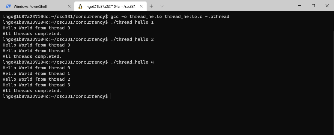
9. Hands on: threads and gdb

Recompile thread_hello.c with gdb support, then run gdb:
$ gcc -g -o thread_hello thread_hello.c -lpthread
$ gdb thread_hello
We will set the breakpoint to the thread function myThreadFun, then run the program with one command line argument.
gdb-peda$ b myThreadFun
gdb-peda$ run 2
We are inside a thread

Run i threads to see how many threads there are in total.

Then run thread apply all bt to learn more about the threads.

There are a total of three threads. Thread 1 comes from the main process. The other two threads (2 and 3) where created from the pthread_create function call.

The numbered sections under the threads represent the stack frames.
gdb-peda$ i threads
gdb-peda$ thread apply all bt
The outcomes of the previous command shows the stack frames of each thread.

We can use thread i to switch to thread i, then frame j to switch to the j^th of that thread.

i locals will print out all local variables of the current stack frame.

Continue running the followings:
gdb-peda$ thread 1
gdb-peda$ i locals
gdb-peda$ frame 1
gdb-peda$ i locals
gdb-peda$ frame 3
gdp-peda$ i locals
When a thread is created, the main process also turns into a management thread and holds to wait for the child threads to finish (pthread_join). Each thread (including the main thread) is located a segment on stack.

We can use thread apply i a_command to apply a_command to thread i.

Let’s advance thread 2 to next commmand:
gdb-peda$ thread 3
gdb-peda$ thread apply 3 n
gdb-peda$
Scroll up a bit and observe. You will see a thread exited. Which thread is this?

What happened?

Switch back to thread 1, continue running n until you are back to the main process.

Keep running n to finish the program.

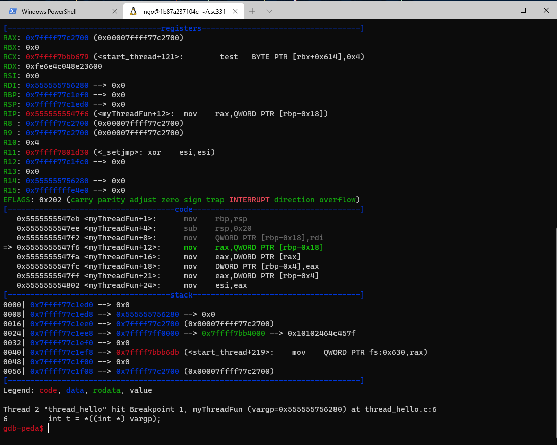
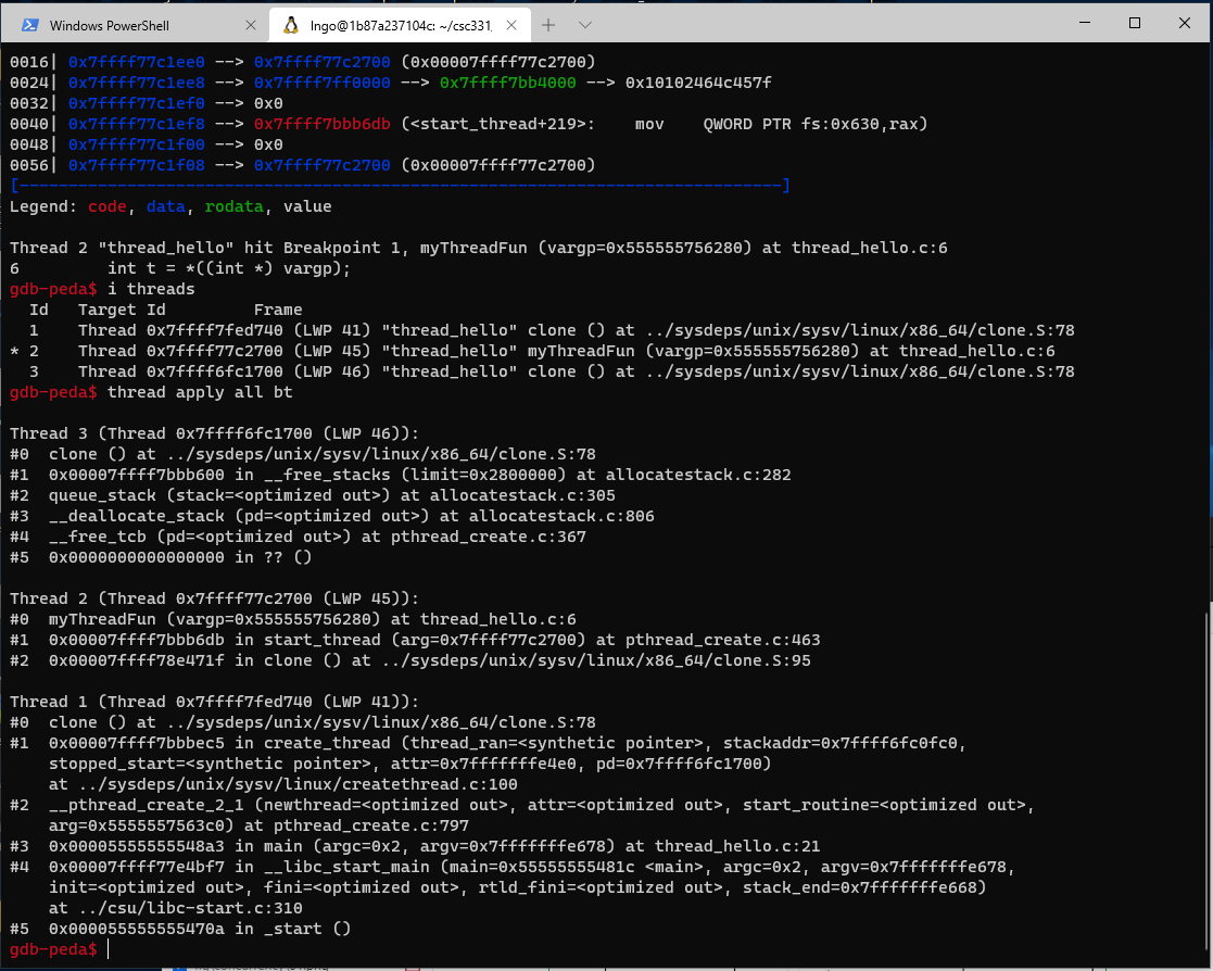
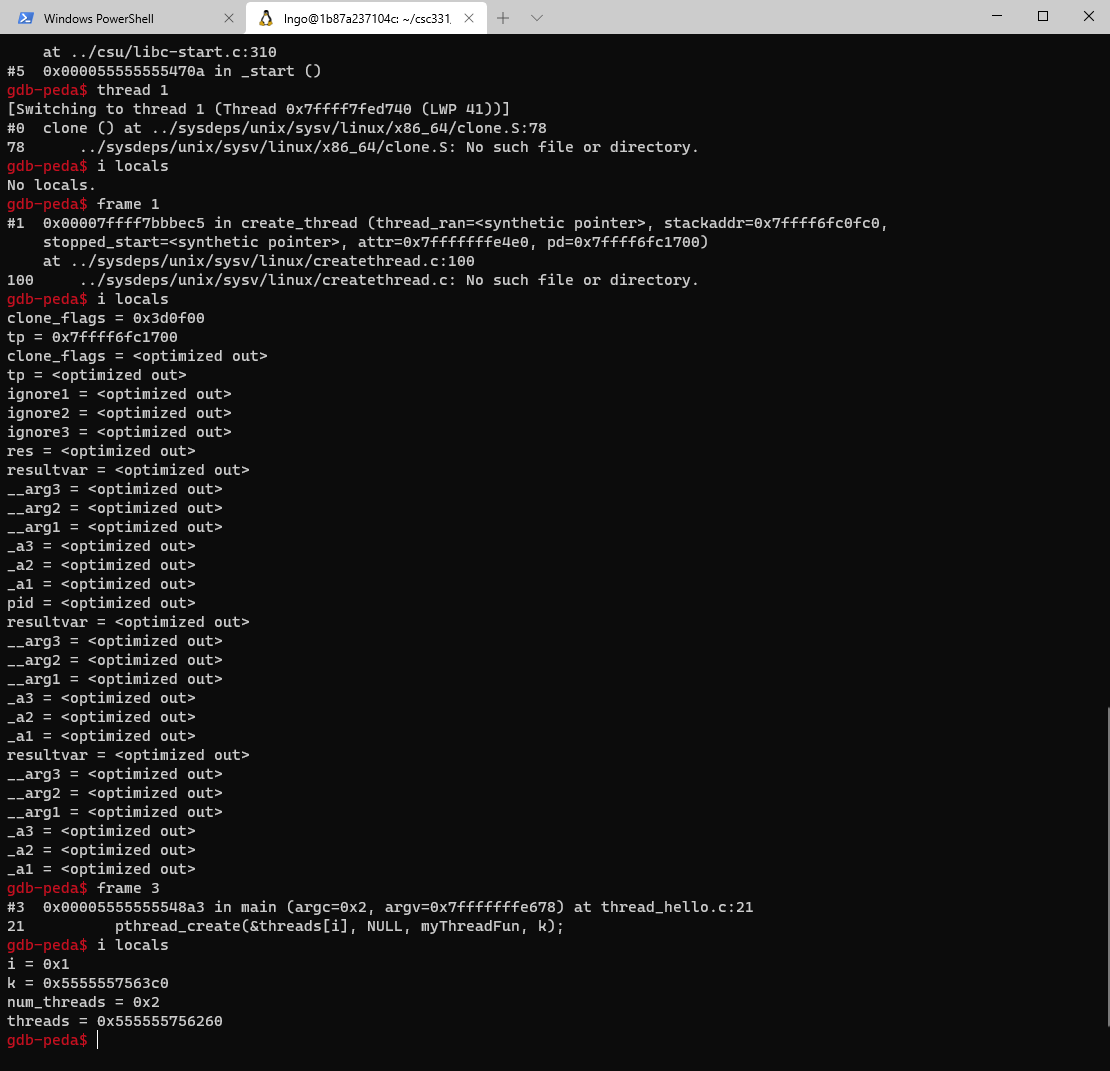
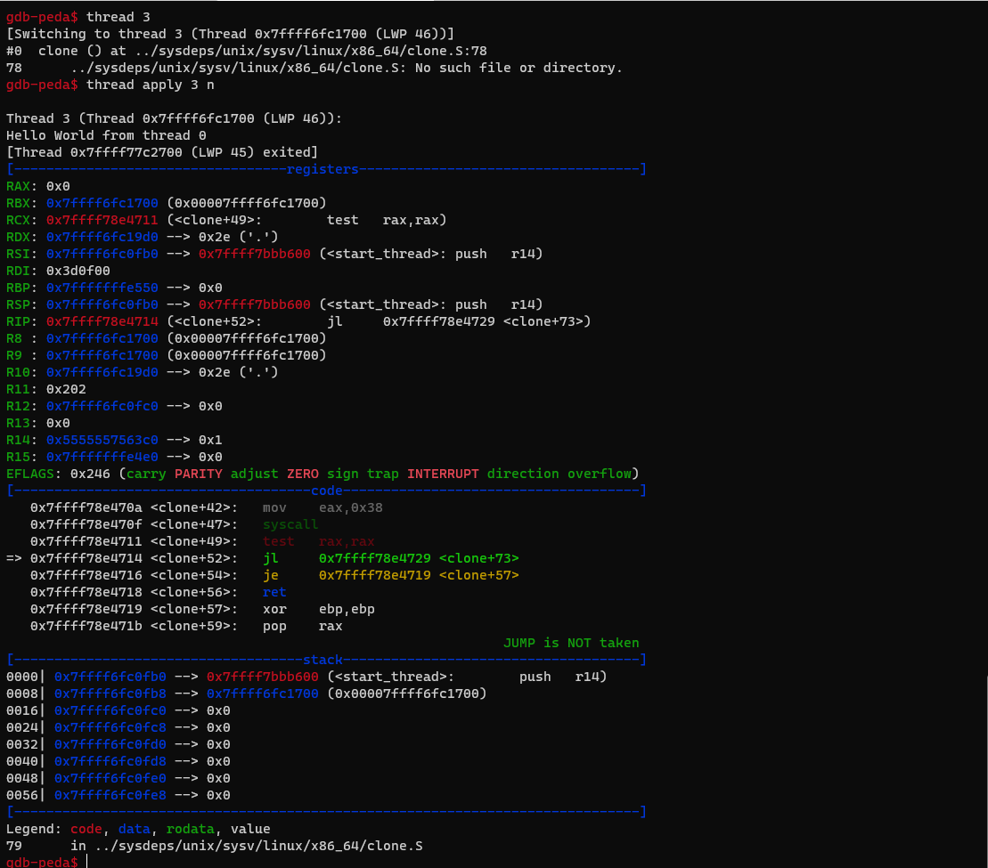
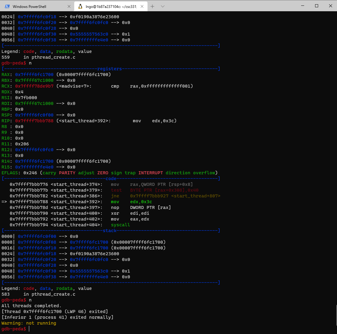
10. The problem with threads

Edward Lee (2006). “The Problem with Threads”. Computer 39(5).

From a fundamental perspective, threads are seriously flawed as a computation model because they are wildly nondeterministic… The programmer’s job is to prune away that nondeterminism. We have developed tools to assist in the pruning: semaphores, monitors, and more modern overlays on threads offer the programmer ever more effective pruning. But pruning a wild mass of brambles rarely yields a satisfactory hedge. To offer another analogy, a folk definition of insanity is to do the same thing over and over again and expect the results to be different. By this definition, we in fact require that programmers of multithreaded systems be insane. Were they sane, they could not understand their programs.`

11. Challenge

Inside concurrency, change to this directory, and create thread_matrix.c with the following contents:

Compile thread_matrix.c with -g then run the program inside gdb with the breakpoint set to the matrix_mul function.

The run command should accept 4 as a command line argument.

Perform the following tasks:

Identify the index of the first C cell on which thread 3 will operate ?

Check the value inside this index from thread 2.

Inside thread 3, advance until the value inside this cell has been modified.

Check that the value from thread 2 is modified as well.

Also check that values of start and end are different inside 2 and 3.

Key Points

First key point. Brief Answer to questions. (FIXME)

Lock and Condition Variables

Overview

Teaching: 0 min
Exercises: 0 min

Questions

How to support atomicity with locks and condition variables?

Objectives

First learning objective. (FIXME)

1. Recall the problem from intro-to-os

Two concurrent threads manipulated a shared resource (the counter variable) without any synchronization.

Outcome depends on the order in which accesses take place – this is called a race condition.

We need to ensure that only one thread at a time can manipulate the shared resource so that we can reason about program behavior, in a sane way

We need synchronization.

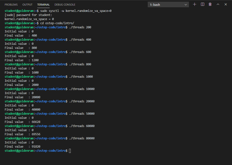
2. What is shared/not shared in a multithreaded program?

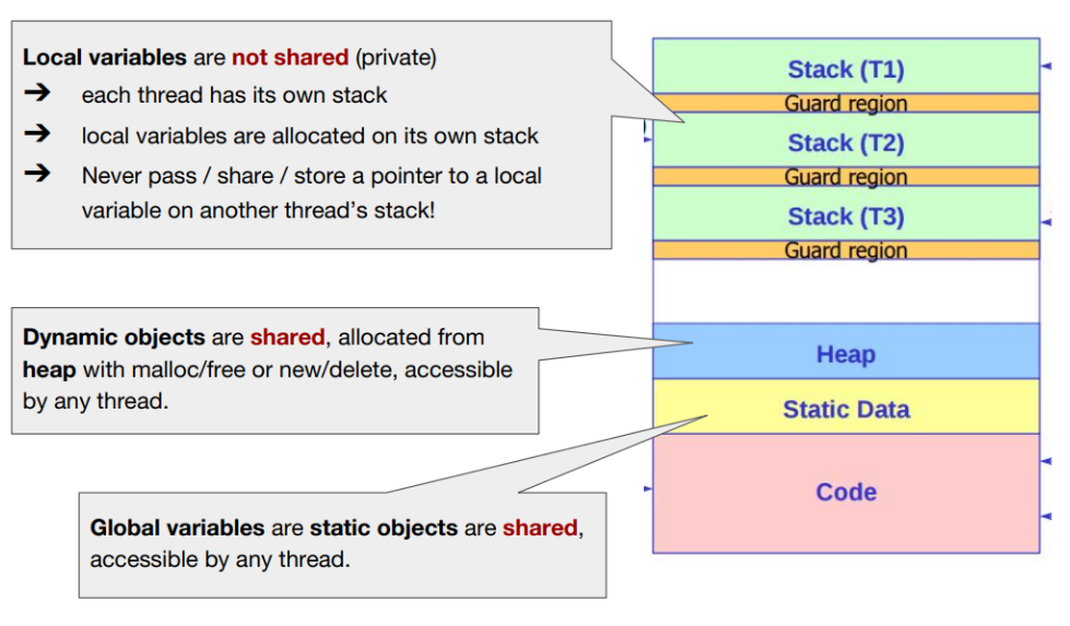
3. Key definitions

A critical section (CS) is a segment of code that accesses a shared resource, usually a variable or data structure.

A race condition (data race) arises if multiple threads of execution enter the critical section at roughly the same time; both attempt to update the shared data structure, leading to a surprising and undesirable outcome.

An indeterminate program consists of one or more race conditions. The outcome is thus not deterministic.

To avoid these problem, threads should use some kind of mutual exclusion primitives. Doing so guarantees that only a single thread ever enters a critical section, thus avoiding races and resulting in deterministic program outputs.

4. Requirements for Critical Section Handling

Mutual Exclusion: if one thread is in the CS, then no other is

Progress: threads waiting for access to CS are not prevented from entering by threads not in the CS; threads do not wait indefinitely.

Bounded Waiting (no starvation): all waiting threads are guaranteed to eventually get access to the CS.

Performance: The overhead of entering and exiting the CS is small compared to the work done within it.

5. Lock: Definition

Atomic instruction: A machine instruction that can be executed in a single clock cycle.

Programmers annotate source code with locks around a critical section, ensuring that it behaves like a single atomic instruction.

What is a lock?

Is declared as a lock variable.

The lock variable holds the state of the lock.

The states are either:

Available (unlocked or free): No thread holds the lock

Acquired (locked or held): Exactly one thread holds the lock and presumably is in a critical section.

The lock variable can also hold additional information (often hidden from users):

Which thread is holding the lock

A queue for ordering lock acquisition …

6. Semantic of locking: lock() and unlock()

A thread calls lock() when it tries to acquire the lock:

If no other thread is holding the lock, the thread will acquire the lock and enter the critical section (becomes owner of the lock).

If another thread is holding the lock, the call will not return.

Once the lock owner is finished, it calls unlock() and the lock becomes available.

If there is no waiting thread, the lock becomes free.

If there are some waiting threads, one of them will acquire the lock and enter the critical section.

Lock in pthread: https://linux.die.net/man/3/pthread_mutex_lock

7. How do we build a lock?

How do we build an efficient lock?

What hardware support is needed?

What OS support is needed?

8. Criteria of a good lock

Mutual exclusion

Fairness

Performance

9. First attempt: controlling interrupts

One of the earliest solutions for single processor systems.

lock() will disable interrupts.

unlock() will enable interrupts.

Advantages

Simplicity

Disadvantages

Allow user programs to perform privileged operations

Disable interrupts carries significant implication in preventing OS from performing interventions.

Do not work on multi-processors (since another thread can still enter the critical section via different computing core).

Prevent non-locking interrupts to take place. For example, disk I/O interrupts.

Inefficient. It is difficult to implement code that mask/unmask interrupts.

10. We need CPU hardware support

Simple principle: Load and Store a lock flag

Correctness:

Interrupts can still lead to inconsistency issues

Performance:

The waiting threads need to keep checking the condition of the flag (spin-waiting)

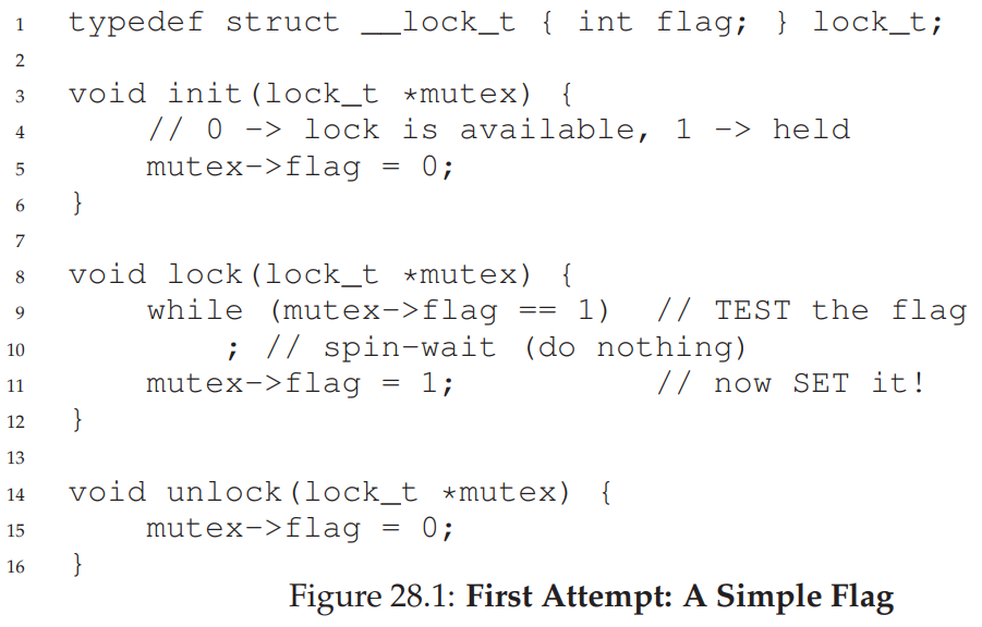
11. Spin lock with Test-and-Set

Hardware support for locking begins in early 1960.

TestAndSet can be performed atomically by hardware.

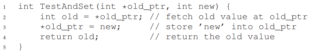
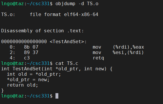
12. Spin lock with Test-and-Set: how does it work?

Lock is free:

flag is 0

TestAndSet returns the old value of flag (break the loop) but also set the value of the flag (acquire the lock).

Lock is not free:

flag is 1

TestAndSet keeps setting the lock but also spinning inside the while loop until the lock is released.

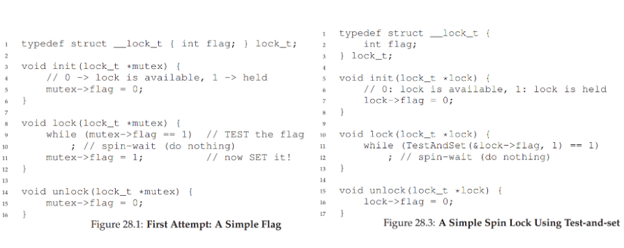
13. Evaluating the basic spin lock

Correctness: Yes

Fairness: No - can lead to starvation

Performance:

TestAndSet requires CPU cycle (even as an atomic operation)

14. Scenario: one thread waiting on another

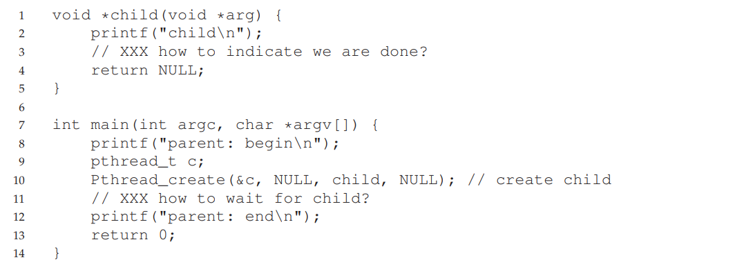
15. A lock-based solution

How to implement a lock-based solution?

What is the issue?

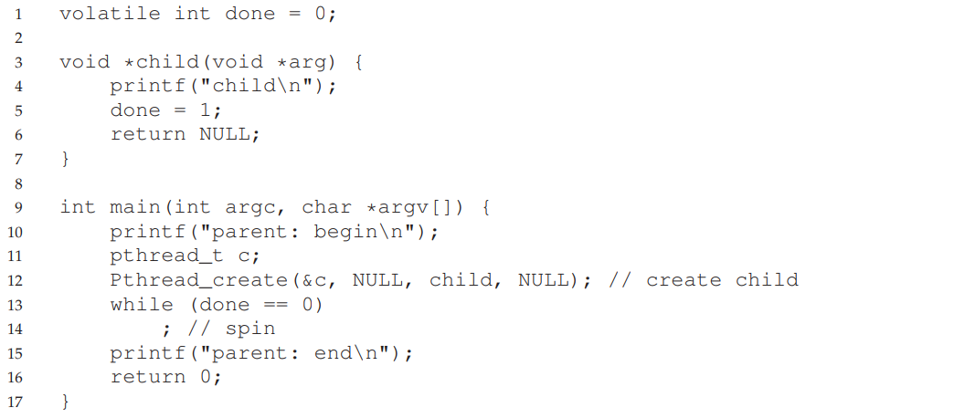
16. How to wait for a condition?

Condition Variable: an explicit queue that threads can put themselves on when some state of execution (condition) is not as desired (waiting on the condition).

When the state is changed, the condition variable can wake up one (or more) of the waiting threads to continue.

pthread_cond_wait

pthread_cond_signal

17. Lock and conditional variable

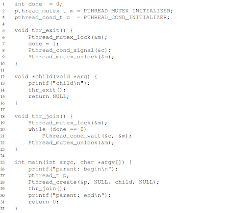
18. Do we really need both?

Infinite sleep for parent thread.

Why?

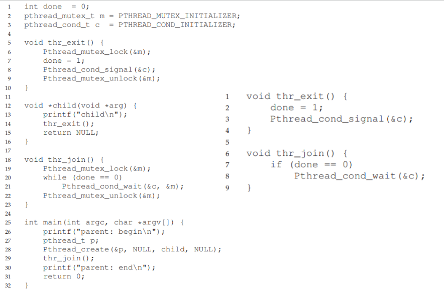
19. The producer/consumer (bounded buffer) problem

Proposed in 1972 by Edsger W. Dijkstra

Imagine one or more producer threads and one or more consumer threads.

Producers generate data items and place them in a buffer;

Consumers grab said items from the buffer and consume them in some way.

Occurs in many real systems

Multi-threaded web servers

Linux pipe

Generalization: many producers/consumers running concurrently.

Requirement:

Only place data in buffer when count is 0 (available space on buffer)

Only grab data from buffer when count is 1 (buffer is full)

20. Vanilla: not thread-safe

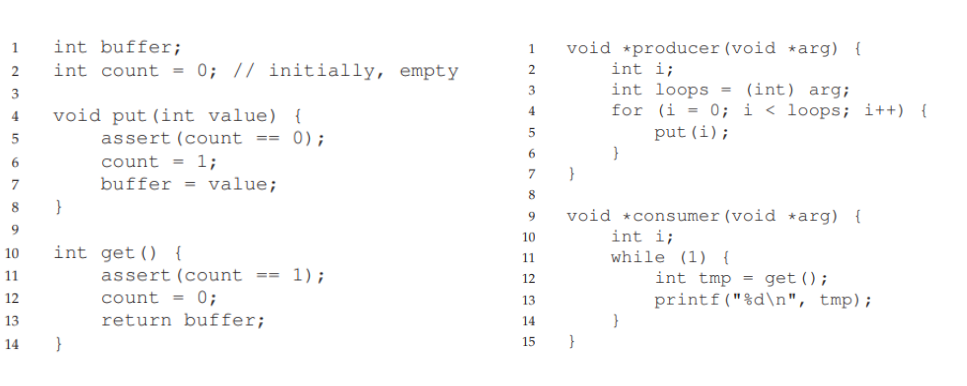
21. First implementation

Start with 1 CV and 1 lock.

Work with 1 producer and 1 consumer.

What happens if we have more consumers?

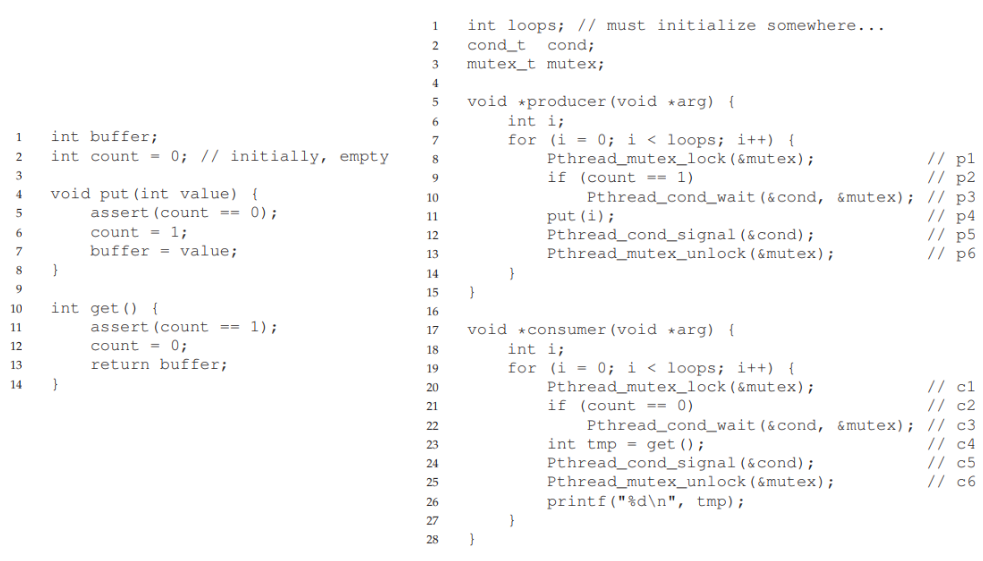
22. First implementation: broken

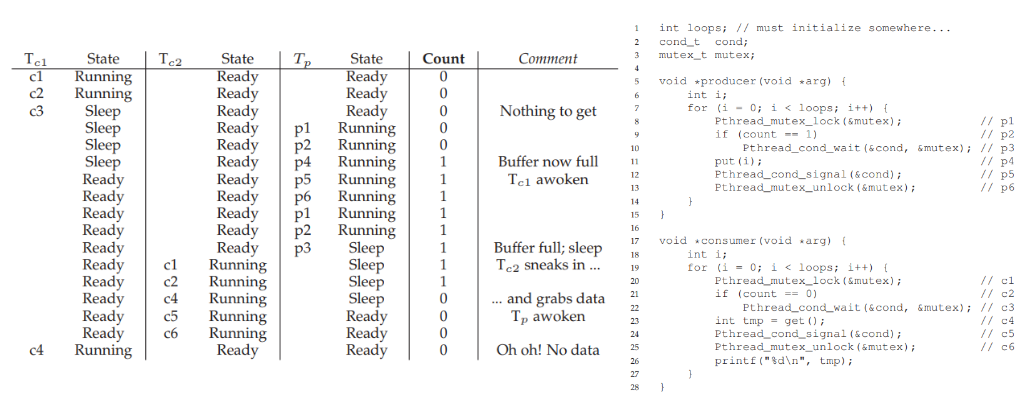
23. First implementation: why?

After the producer wakes a consumer, the state of bound buffer changed for the consumer due to the other consumer.

Signaling a state only wakes them up (implying a state changes) but does not guarantee maintaining a desired state.

This is called Mesa semantics

“Experience with Processes and Monitors in Mesa” by B.W. Lampson, D.R. Redell. Communications of the ACM. 23:2, pages 105-117, February 1980

Virtually all computing systems are built using Mesa semantics.

Hoare semantics

Stronger guarantee that the woken thread will run immediately upon being woken.

24. Second implementation: slightly less broken

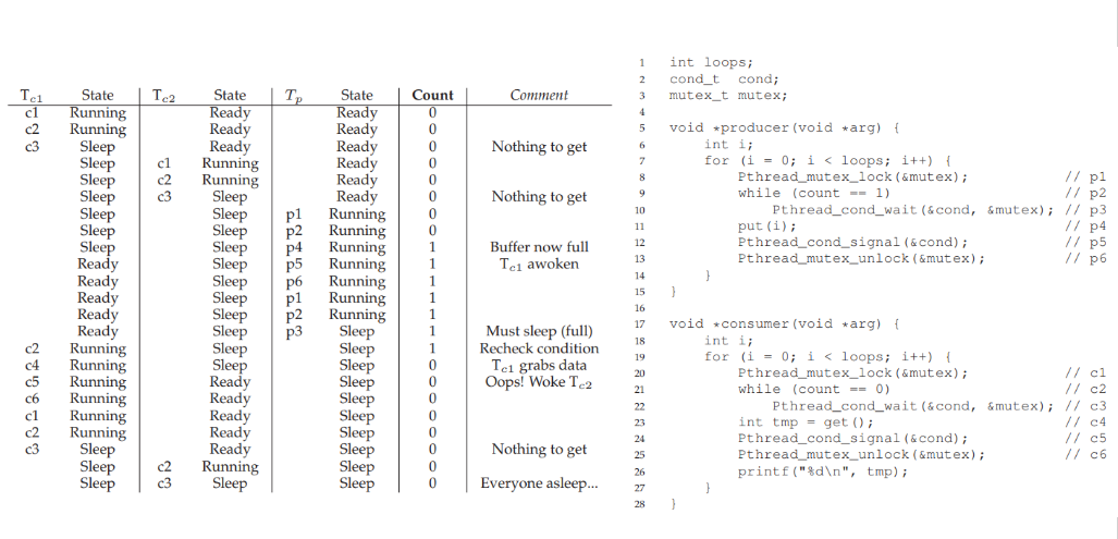
25. Third implementation: finally work

Consumer only wake producer and vice versa

Two condition variables are needed.

Not yet generalized.

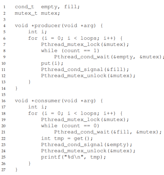
26. A generalized solution

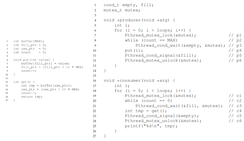
Key Points

First key point. Brief Answer to questions. (FIXME)

Semaphores

Overview

Teaching: 0 min
Exercises: 0 min

Questions

How to support atomicity with semaphores?

Objectives

First learning objective. (FIXME)

1. What have we learned so far?

Both lock and condition variables are needed to solve more complex concurrency problems.

Can we do better?

2. Edsger Dijkstra

Dijkstra, Edsger W. “The structure of the “THE” multiprogramming system.” In The origin of concurrent programming, pp. 139-152. Springer, New York, NY, 1968.

Dijkstra, Edsger W. “Information streams sharing a finite buffer.” In Inf. Proc. Letters, vol. 1, pp. 179-180. 1972.

Together with colleagues, developed semaphore as a single primitive for all things related to synchronization.

3. Semaphore

Is an object with an integer value that can be manipulated with two routines:

sem_wait()

sem_post()

Needs to be initialized to some value.

sem_init()

3. sem_wait() and sem_post()

More important, how do we use sem_wait() and sem_post() to facilitate synchronization for concurrency?

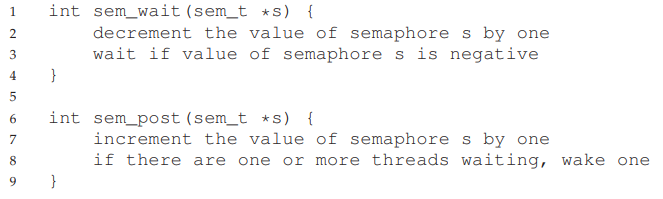
4. Aspects of sem_wait() and sem_post()

sem_wait() and sem_post() are atomic operations.

sem_wait() either return right away or it will cause the caller to wait.

sem_post() simply increase the value of the semaphore and wakes one of the waiting thread up.

The value of the semaphore, when negative, is equal to the number of waiting threads.

5. Semaphore as lock (binary semaphore)

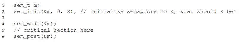
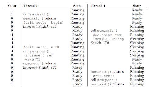
6. Semaphore as condition variable

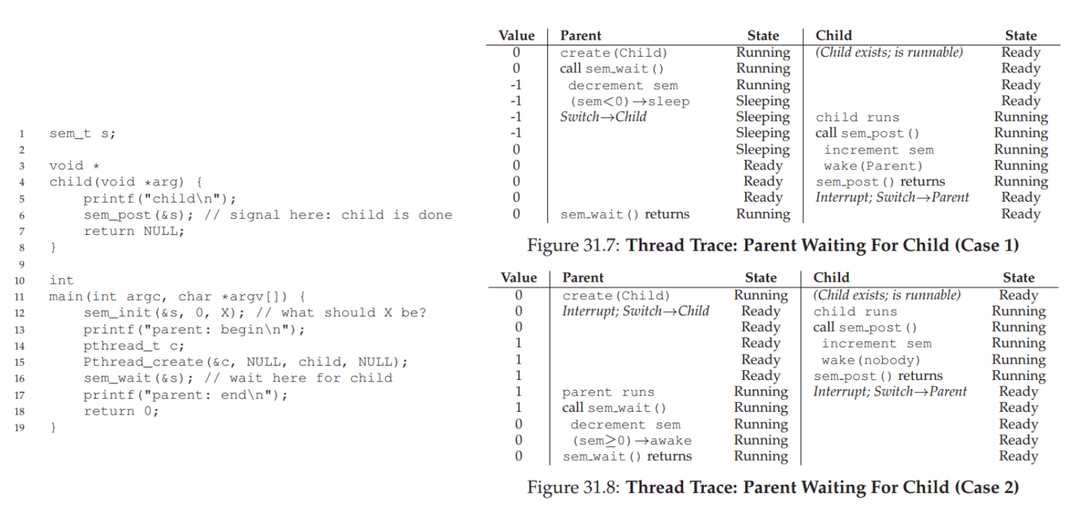
7. Semaphore: producer/consumer I

What is the risk if MAX > 1 and there are multiple producers/consumers?

Race condition: two producers produce at the same time or two consumers consume at the same time.

What is currently missing from this implementation?

Mutual exclusion

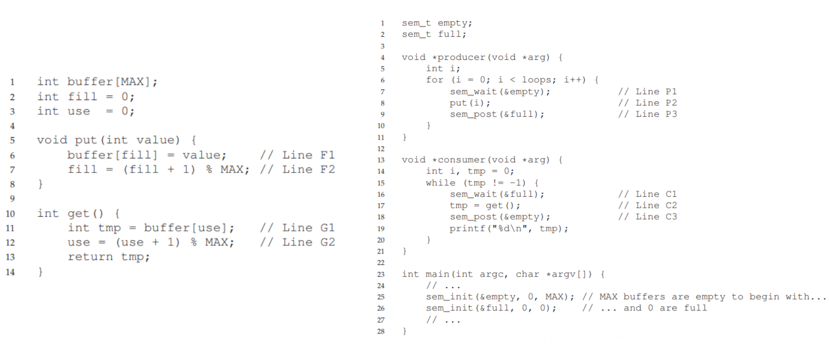
8. Semaphore: producer/consumer II

Mutual exclusion is added, incorrectly.

Consumer runs first, then wait on full (but still holding mutex).

Producer sees negative mutex, decreases it further, then goes to sleep.

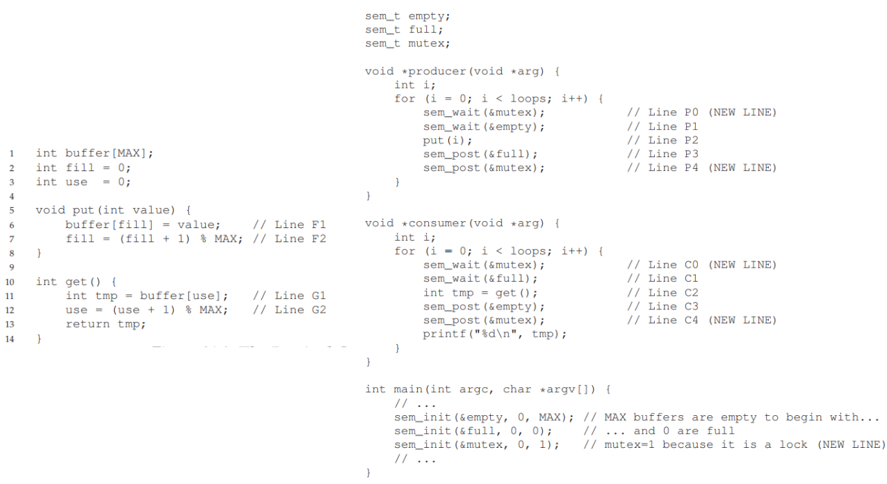
9. Semaphore: producer/consumer III

Mutual exclusion is added, correctly.

full and empty are for producers and consumers to wait on one another.

mutex for producers and consumers to wait among each group.

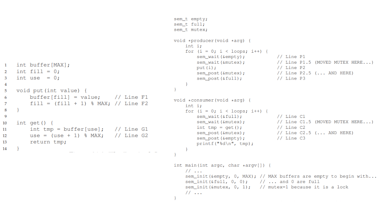
10. The dining philosophers

It’s Dijkstra again.

There are five philosophers seating around a table.

Between each pair of philosophers there is a single fork (five forks total).

Philosophers alternate between thinking and eating (need fork).

Two forks are needed to eat (one to the left and one to the right).

How to schedule fork grabbing pattern so that no one starves?

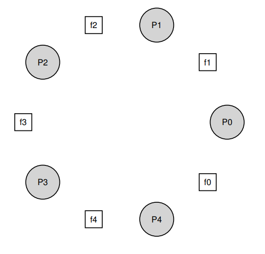
11. Solutions

which one works?

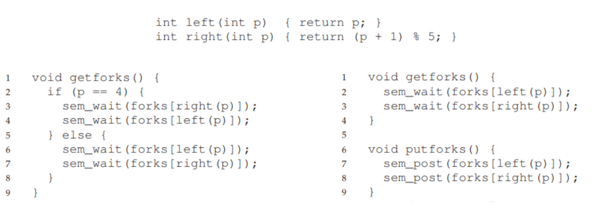
Key Points

First key point. Brief Answer to questions. (FIXME)

I/O and Disks: Disk Scheduling

Overview

Teaching: 0 min
Exercises: 0 min

Questions

How to access data on disk?

Objectives

First learning objective. (FIXME)

1. Input/Output devices

Critical to computer systems

Without input: Same results every time.

Without output: What’s the point?

How should I/O be integrated into systems?

What are the general mechanisms?

How can we make them efficient?

2. Classical system architecture

Hierarchical structure due to the relationship between physics and costs:

The faster the bus, the shorter it is.

The faster the bus, the more complex it is to design and build (hence more costly).

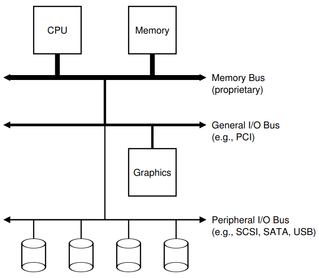
3. Modern system architecture

Specialized chipsets and faster point-to-point interconnects.

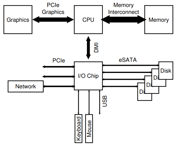
4. Canonical device

Interface: allowing system software to control the device’s operations

Internal structure: implementing the abstraction presented to the system.

Abbreviations:

DMI: Direct Memory Interface

ATA: IBM’s PC AT Attachment.

SATA: Serial ATA

eSATA: External Serial ATA

PCIe: Peripheral Component Interconnect Express

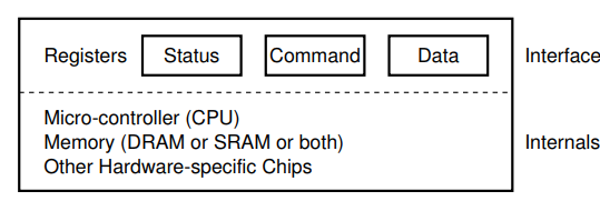
5. A simple canonical protocol

Repeatedly read the register for READY status.

Send data to register (Programmed I/O - PIO).

Write a command to the command register to initiate device execution.

Wait until the device is done.

What is a problem with this approach?

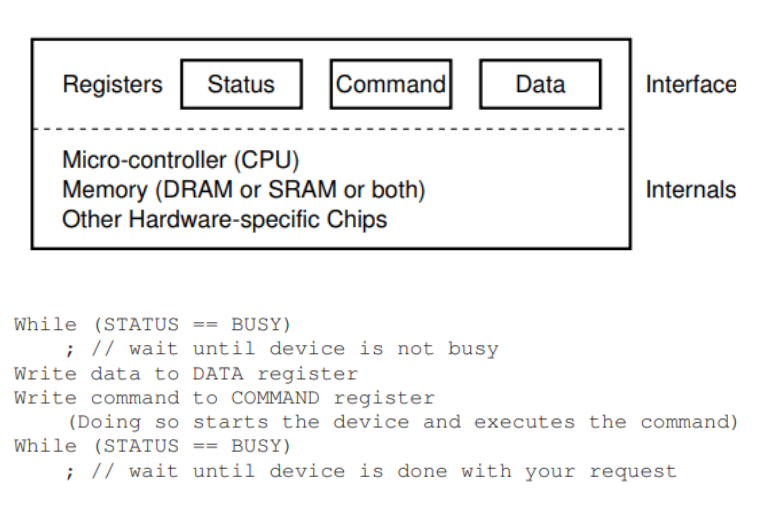
6. Hardware interrupts

Instead of polling the device, the OS can:

After issue an I/O request, put the calling process to sleep and context switch to another.

When the request is finished, the device will raised a hardware interrupt to return CPU to the OS.

Predetermined interrupt service routine (ISR) - interrupt handler.

This allows overlap of computation and I/O (recall CPU scheduling slides)

To avoid interrupts all the time, a hybrid model is employed (scheduling).

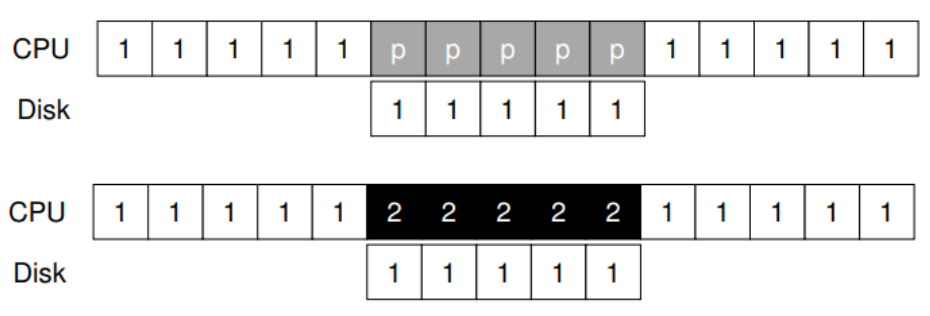
7. Programmed I/O overheads

Programmed I/O: I/O instructions that move data from storage into register for computation purposed. This requires the CPU’s involvement in every transactions.

With programmed I/O, the CPU spends too much time moving data to and from devices.

How do we offload this work: Direct Memory Access (DMA) device

Orchestrate transfer between devices and main memory without much CPU intervention.

Example: Intel Broadwell Crystal Beach DMA Application

Supports write operations from memory to I/O, but not from I/O to memory

Instantiated as a root complex integrated PCIe end-point device

Chipset DMA that is controllable by software executing on the processor

A standardized software interface for controlling and accessing DMA features

There are eight software visible CB DMA engines, visible as PCI functions.

Each engine has one channel.

Each can be independently operated.

In a virtualized system, each can be independently assigned to a VM.

Copying of data is handled by DMA controller.

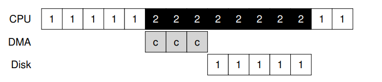
8. Method of device interaction

First method

Explicit I/O instructions (privileged)

Second method

Memory-mapped I/O

The hardware makes the device registers available as if they were memory locations.

No clear advantages on either method

9. Device driver

How to fit various I/O devices with different interfaces into the OS (which is supposed to be generic)?

Abstraction, abstraction and abstraction: device driver

70% of OS code is found in device drivers.

Unofficial device drivers are often the cause for kernel crashes.

Example:

AMD Device Driver for Vulkan

API guide for Linux driver implementation

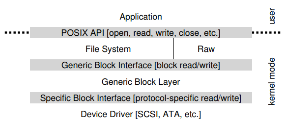
10. Disk Drive

Large number of sectors (512-byte blocks)

Sectors are numbered 0 to n-1 on disks with n sectors. This is the address space of the drive.

Multi-sector operations are possible (read or write 4K bytes at a time).

Only a single 512-byte write is guaranteed atomic.

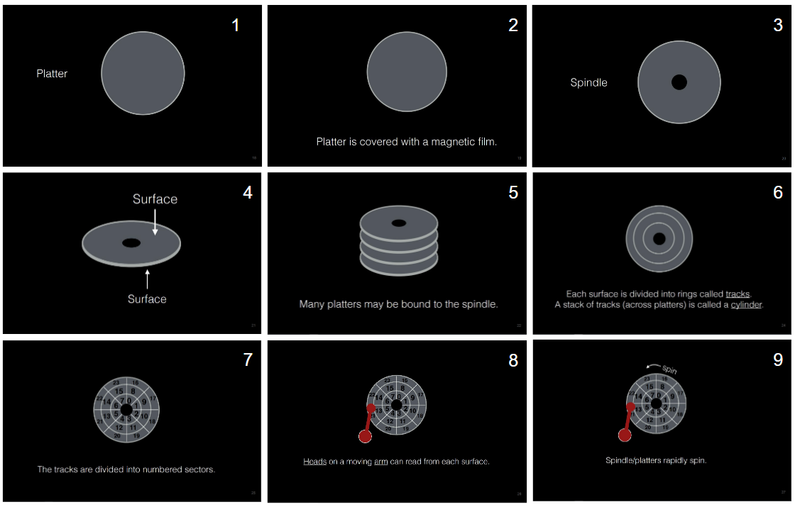
11. Seek, rotation, transfer

Seek: move the disk arm to the correct cylinder

depends on how fast disk arm can move

typical time: 1-15ms, depending on distance (average 5-6ms)

improving very slowly: 7-10% per year

Rotation: waiting for the sector to rotate under the head

depend on the rotation rate of the disk (7200 RPM SATA, 15K RPM SCSI)

average latency of ½ rotation (~4ms for 7200 RPM disk)

has not changed in recent years

Transfer: transferring data from surface into disk controller electronics, or the other way around

depends on density, higher density, higher transfer rate

~100MB/s, average sector transfer time of ~5 microseconds

improving rapidly (~40% per year)

12. Disk scheduling

The OS has a queue of disk requests, therefore there is a chance to schedule these requests

We want to minimize seeking

13. Disk scheduling algorithms

FCFS (do nothing)

reasonable when load is low, long waiting time when load is high

SSTF (shortest seek time first)

minimizes arm movement

favors blocks in middle tracks, because they have more blocks nearby.

SCAN (elevator)

serve request in one direction until done, then reverse

like an elevator, avoid going back and forth in the middle

C-SCAN (typewriter)

like SCAN, but only go in one direction (no reverse direction)

LOOK / C-LOOK

like SCAN/C-SCAN, but only go as far as last request in each direction, instead of going full width of the disk.

Disk scheduling is important only when disk requests queue up

important for servers

not so much for PCs

Modern disks often do disk scheduling themselves

Disks know their layout better than the OS, can optimize better

on-disk scheduling ignores, undoes any scheduling done by the OS

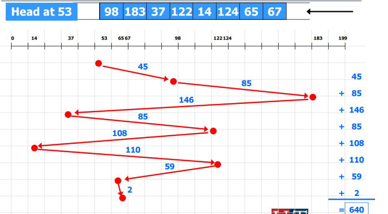
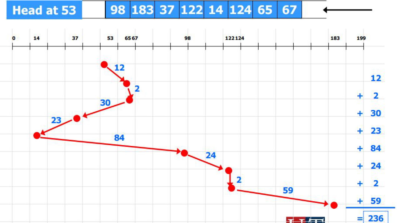
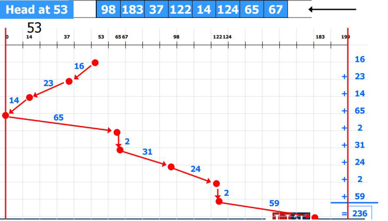
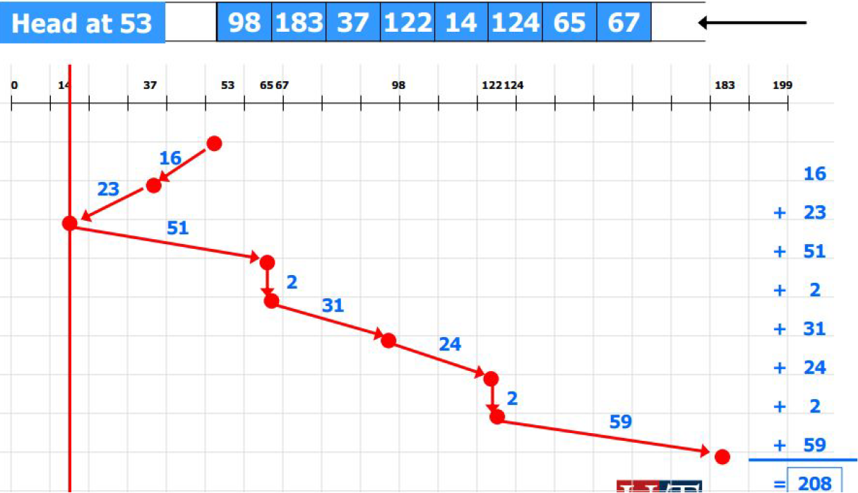
Key Points

First key point. Brief Answer to questions. (FIXME)

Introduction to file systems

Overview

Teaching: 0 min
Exercises: 0 min

Questions

How to manage a persistent device?

How to implement a simple file system?

Objectives

First learning objective. (FIXME)

1. File systems

Provide long-term information storage

Challenges:

Store very large amounts of information

Multiple processes must be able to access ino concurrently

Information must survive (persist)

termination of process using it

computer crashes

disk failures

power outage

…

Easy-to-use user interface

2. Files and directories

It’s all illusion!

CPU virtualization: a process that has its own processor.

Memory virtualization: a big, contiguous, and private address space that can easily be accessed through virtual addresses.

Storage virtualization: a huge, persistent storage with files and directories which can be accessed using some easy-to-use APIs (ls, rm, cp …).

3. Abstraction: files and directories

File: a linear array of bytes, each of which you can read and write.

A file has some high-level, user-readable name, e.g., interceptor.c.

One file may have multiple user-readable names, as we will see.

Each file has a low-level name called the inode number.

This is the real identifier of a file.

File system does NOT care about what type of file it is (C code, picture or video, it just makes sure to store all bytes in a file persistently.

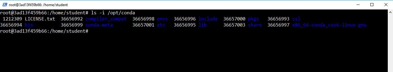
4. Abstraction: files and directories

Directory

Each directory also has an inode number

Content of a directory:

a list of (user-readable name, inode number) pairs

which are the files and directories under this directory

Directory tree / hierarchy

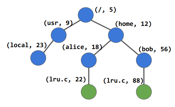
5. File operations: create

create: int fd = open(“foo”, O_CREAT | O_WRONLY | O_TRUNC, S_IRUSR | S_IWUSR)

open

O_CREAT: creates the file if it does not exist.

O_WRONLY: the file can only be written to.

O_TRUNC: if the file already exists, truncates it to zero bytes, removing any existing contents.

S_IRUSR: readable by the owner,

S_IWUSR: writable by the owner.

fd: file descriptor, starts at 3 ( Reserved values: 0 for stdin, 1 for stdout, 2 for stderr)

read: ssize_t read(int fd, void *buf, size_t count)

read

fd: file descriptor value

*bf: memory address to store data read from file represented by fd.

count: number of bytes to be read

A successful read will return the number of bytes read or a -1 if there is an error.

write: ssize_t write(int fd, const void *buf, size_t count)

write

fd: file descriptor value

*bf: memory address containing data to be written to the file represented by fd.

count: number of bytes to be written.

A successful write will return the number of bytes written or a -1 if there is an error.

6. Hands on: file operations

Before turning on the VM, makes sure that you have two processors assigned to your VM.

Open a terminal (Windows Terminal or Mac Terminal).

Run the command to launch the image container for your platform:

Windows:
$ podman run --rm --userns keep-id --cap-add=SYS_PTRACE --security-opt seccomp=unconfined -it -v /mnt/c/csc331:/home/$USER/csc331:Z localhost/csc-container /bin/bash
Mac:
$ docker run --rm --userns=host --cap-add=SYS_PTRACE --security-opt seccomp=unconfined -it -v /Users/$USER/csc331:/home/$USER/csc331:Z csc-container /bin/bash
Root password: goldenrams
$ sudo apt-get install -y strace
$ echo "Hello World" > hello.txt
$ strace -t -o cat_log cat hello.txt 
$ cat cat_log
Search the manual of the following functions: openat, fstat, fadvise64, and mmap.

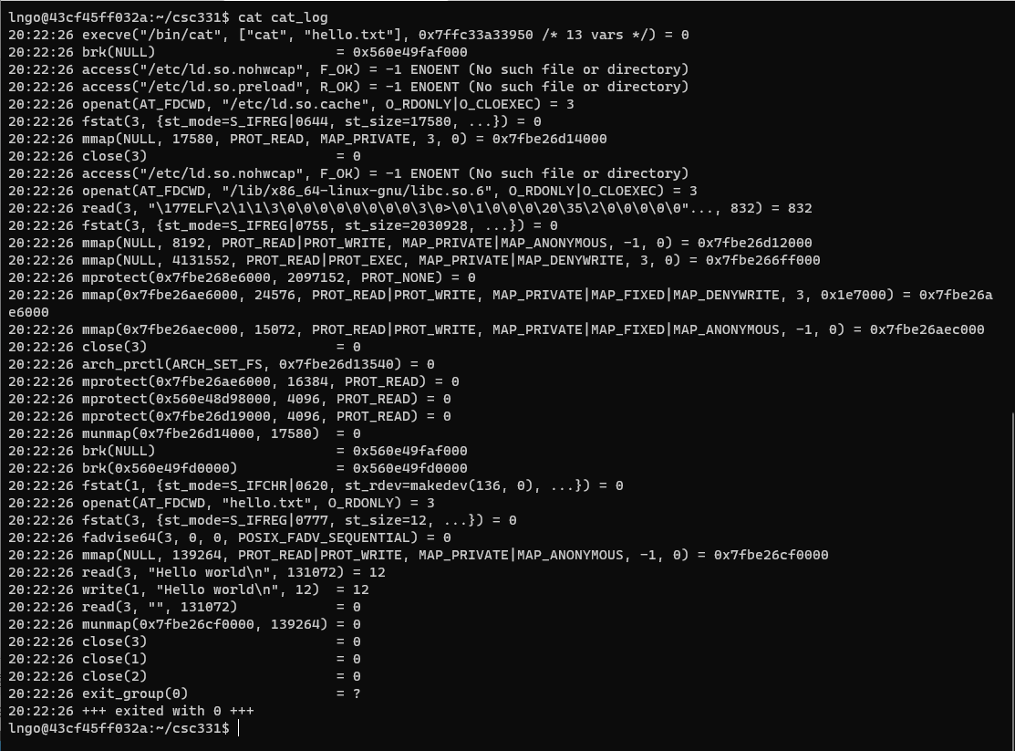
7. Non-sequential read/write: lseek

read() and write() only do sequential read/write, there is no way to specify a particular read/write position (offset).

For each file opened by a process, the OS keeps track of a current offset, which determines where the next read/write happens, read() and write() updates current offset according to how many bytes are read/written

cannot update current to wherever they want

If want to update current to wherever you want, use lseek(): off_t lseek(int fd, off_t offset, int whence)

lseek

fd: file descriptor valur

offset: offset value.

whence:

if whence is SEEK_SET, the current offset is set to offset bytes

if whence is SEEK_CUR, the current offset is set to current + offset bytes

if whence is SEEK_END, the current offset is set to size_of_file + offset bytes

8. Implementations of file systems

There exist many, many file system implementations, literally from AFS to ZFS.

File system implementations

Some famous ones:

FAT32, NTFS used by Windows

HFS+ used by Mac OS X

UFS, ZFS used by BSD, Solaris

ext2, ext3, ext4, ReiserFS, XFS, JFS used by Linux

We will study a very simple example file system named VSFS: Very Simple File System

Analogy

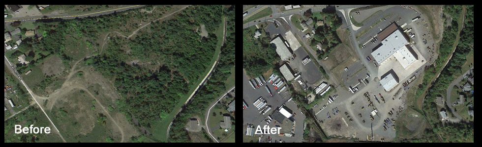
9. How to implement a simple file system?

What structures are needed on the disk?

What do they need to track?

How are they accessed?

10. Mental model of a file system

What on-disk structures store the file system’s data and metadata?

What happens when a process opens a file?

Which on-disk structures are accessed during a read or write?

By working on and improving your mental model, you develop an abstract understanding of what is going on, instead of just trying to understand the specifics of some file-system code (though that is also useful, of course!).

Unformatted raw disk

Overall organization

The whole disk is divided into fixed-sized blocks.

Block size: 4KB

Number of blocks: 64

Total size: 256KB

Data region

Most of the disk should be used to actually store user data, while leaving a little space for storing other things like metadata

In VSFS, we reserve the last 56 blocks as data region.

Metadata: inode table

The FS need to track information about each file.

In VSFS, we keep the info of each file in a struct called inode. And we use 5 blocks for storing all the inodes.

Maximum number of inodes it can hold: 5 * 4KB / 128B = 160, i.e., this VSFS can store at most 160 files.

Allocation structure

For both data region and inode region, we need to keep track of which blocks are being used and which blocks are free.

We use a data structure called bitmap for this purpose, which is just a sequence of bits, and each bit indicates whether one block is free (0) or in-use (1).

We have one bitmap for the data region and one bitmap for the inode region, and reserve one block for each bitmap. (4KB = 32K bits, can keep track of 32K blocks)

Superblock

Superblock contains information about this particular file system, e.g.,

What type of file system it is (“VSFS” indicated by a magic number)

how many inodes and data blocks are there (160 and 56)

Where the inode table begins (block 3)

etc.

When mounting a file system, the OS first reads the superblock, identify its type and other parameters, then attach the volume to the file system tree with proper settings.

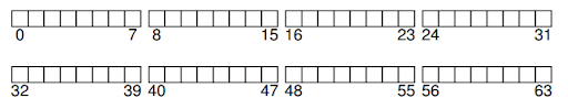
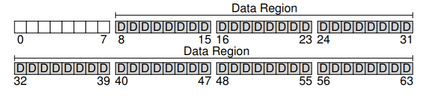
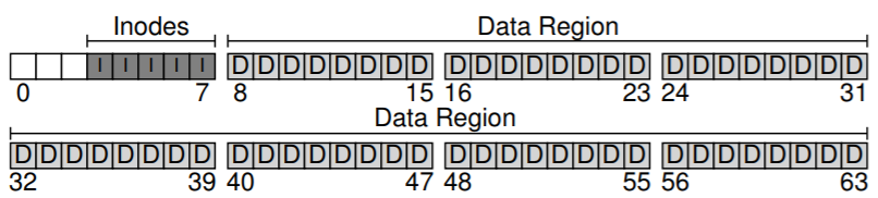
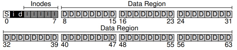
11. Example implementations

xv6 file system

Linux ext2

12. Example: reading a file with inode number 32

From superblock we know

inode table begins at Block 3, i.e., 12KB

inode size is 128B

Calculate the address of inode 32

12KB + 32 * 128B = 16K So we have the inode, but which blocks have the data?

13. Data structure: the inode

Short for index node

In vsfs (and other simple file systems), given an i-number, you should directly be able to calculate where on the disk the corresponding inode is located.

blk = (inumber * sizeof(inode_t)) / blockSize

sector = ((blk * blockSize) + inodeStartAddr) / sectorSize

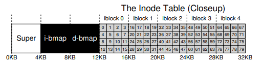
14. Multi-level index with indirect pointers

Direct pointers to disk blocks do not support large files, so people came up with the idea of indirect pointer.

Instead of pointing to block of user data, it points to a block the contains more pointers.

For the 15 pointers we have in an inode, use the first 14 pointers as direct pointers and the 15th pointer as an indirect pointer.

How big a file can we support now?

14 direct pointers in total: 14 data blocks

Indirect pointer points to a block (4KB) which can hold 1K pointers (each pointer is 4B), so 1K data blocks in addition.

So total size supported: 4K * (14 + 1K) = 4152KB

Bigger?

Why use an imbalanced tree like this? Why not a different approach?

Many researchers have studied file systems and how they are used, and virtually every time they find certain “truths” that hold across the decades.

One such finding is that most files are small.

This imbalanced design reflects such a reality: if most files are indeed small, it makes sense to optimize for this case.

A five-year study of file system metadata, 2007

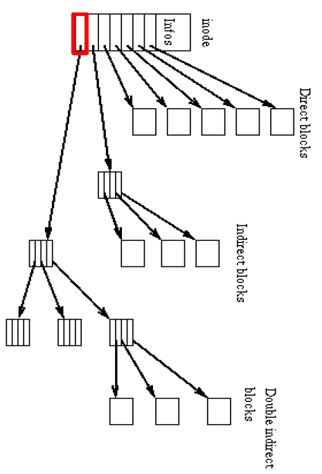
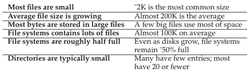
15. Another approach: extent-based

An extent is a disk pointer plus a length (in blocks), i.e., it allocates a few blocks in a row.

Instead of requiring a pointer to every block of a file, we just need a pointer to every several blocks (every extent).

It is less flexible than the pointer-base approach, but uses smaller amount of metadata per file, and file allocation is more compact.

Adopted by ext4, HFS+, NTFS, XFS.

16. Yet anther approach: linked-based

Instead of having pointers to all blocks, the inode just has one pointer pointing to the first data block of the file, then the first block points to the second block, etc.

Works poorly if want to access the last block of a big file. To help, use an in memory file allocation table which is indexed by address of data block, so finding a block can be faster.

This is the FAT file system, used by Windows before NTFS.

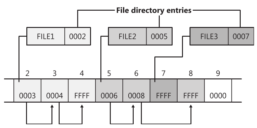
Key Points

First key point. Brief Answer to questions. (FIXME)

Crash consistency: fsck and journaling

Overview

Teaching: 0 min
Exercises: 0 min

Questions

How to update the disks despite crashes?

Objectives

First learning objective. (FIXME)

1. Persistence

Data persists after the computer is powered off

This is a given due to disks’ physics

If the computer crashes during the file system read/write activities, how can we guarantee that data on disk are still consistent?

This is a more interesting problem for operating systems.

The crash-consistency problem

2. A crash scenario

A 4KB file on disk, within a single data block

An additional 4KB is written to the file (one more data block added).

If everything went well:

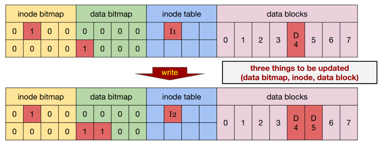
3. If the computer crashed during write

What are all the possible inconsistent states that the FS can be in after the crash?

Only one thing updated

Case 1: Just the data block is updated, but not the data bitmap and inode

Case 2: Just the inode is updated, but but not the data bitmap and data block

Case 3: Just the data bitmap is updated, but not the inode and data block

Only two things updated

Case 4: inode and data bitmap updated, but not data block

Case 5: inode and data block updated, but not data bitmap

Case 6: data bitmap and data block updated, but not inode

4. Case 1: only the data block is updated

The data is on disk

Nobody ever knows, because inode and data bitmap are not updated

The file system itself is still consistent, it is just like nothing happened

No need to fix anything

5. Case 2: only the inode is updated

inode has data block pointer pointing to an unwritten data block

If we trust the inode, we will read garbage data

Also there is inconsistency between data bitmap and the inode:

inode says that the data block #5 is used, but data bitmap say it is not.

if not fixed, could allocate block #5 again and overwrite its data by mistake

6. Case 3: only data bitmap is updated

inode is not pointing data block #5, so no risk of reading garbage data

data bitmap says data block #5 is used, but in fact it is not

data block #5 will never be used again

This is called a space leak.

7. Case 4: Only inode and data bitmap updated

The file system will read garbage data from block #5 again.

The file system doesn’t even realized anything wrong, because the inode and the data bitmap are consistent with each other.

8. Case 5: Only inode and data block updated

The file system will NOT read garbage data.

Data bitmap and inode are inconsistent between each other:

inode says that the data block #5 is used, but data bitmap say it is not

if not fixed, could allocate block #5 again and overwrite its data by mistake

9. Case 6: Only data bitmap and data block updated

Inconsistency between inode and data bitmap.

We know data block #5 is used, but will never know which file uses it

10. Problem!

We wish file system updates were atomic, but they are not.

The there are many different problems that can occur if the computer crashes during a file system update.

Inconsistency in file system data structure

Reading garbage data

Space leak

We call them crash-consistency problems

11. Solution 1: FSCK

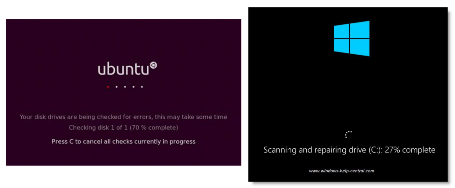
12. FSCK (File System Check)

A UNIX tool that scans the whole disk, finds inconsistencies ands repair them.

It runs before the file system is mounted, e.g., when booting

when crash happens, let it be, and fix it later (when rebooting)

Typical checks performed

all blocks pointed to by inode or indirect block must be marked used in bitmap

all used inodes must be in some directory entry

inode reference count (link count) must match

no duplicate data pointers.

etc.

13. Limitation of FSCK

A working FSCK requires very complicated and detailed knowledge of the file system, and is hard to be implemented correctly.

It only cares about the internal consistency of the file system, and does NOT really care about lost data (e.g., Case 1 and Case 4)

Bigger problem: it is too slow

with a large hard drive, it can easily take hours to finish FSCK

it’s just a bit irrational: scan the whole disk no matter how small an inconsistency needs to be fixed.

14. Solution 2: Journaling (write-ahead logging)

Additional space in the on-disk data structure

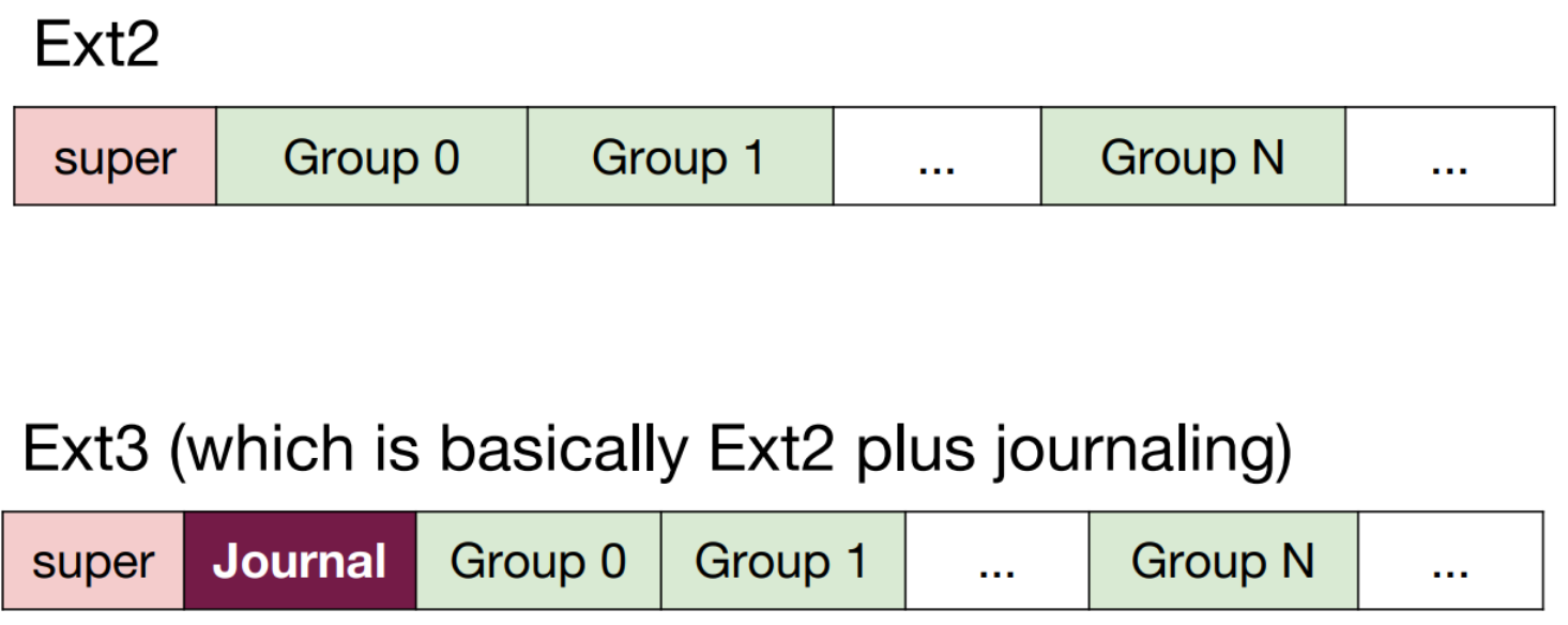
15. Journaling: what to store?

When updating the disk, before making the actual writes to disk, the FS first writes a little note about what it is about to do, to the journal (or log, at well known location on disk).

Failures become recoverable:

If crash happens during actual write (journal write completed), then we can look at the journal and replay the actual writes hence recover the data.

If crash happens even before journal write finishes, then it doesn’t matter since the actual write has NOT happened at all, nothing is inconsistent.

16. Journaling: the structure to be written to the journal/log

Transaction:

starts with a transaction begin (TxB) block, containing a transaction id (TID) followed by blocks with the exact content to be written.

physical logging: putting exact physical content

logical logging: putting more compact logical representation

ends with a transaction end (TxE) block, containing the TID.

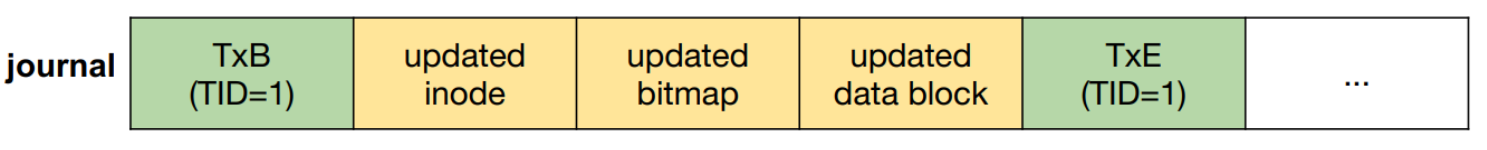
17. Journaling: sequence of operations

Journal write: write the transaction, including the TxB, all pending data and metadata updates, and the TxE, to the journal; wait for these writes to complete.

Checkpoint: actually write the pending data and metadata to to their final locations in the file system.

What can go wrong:

Crash can occur during journal writes.

When having a batch of writes, the disk may perform some disk scheduling, so the writes in the batch can happen in any order.

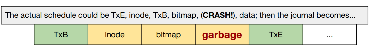
18. Journaling: a better sequence of operations

Journal write: write the transaction, including the TxB, all pending data and metadata updates, NOT including the TxE, to the journal; wait for these writes to complete.

Journal commit: write the TxE block (a.k.a. transaction commit block); now tractions is said to be committed.

Checkpoint: actually write the pending data and metadata to to their final locations in the file system.

Hard disk guarantees atomic write of a 512-byte sector, the TxE block should fit in a 512-byte sector, so the commit is either fully completed or not completed at all.

19. Journaling: recover from a crash

If crash happens before the transaction is committed to the journal/log simply skip the pending update.

If crashed happens during the checkpoint step:

When booting, scan the journal and lookup for committed transactions (much faster than fsck scanning the whole disk).

Replay these transactions.

After replay the file system is guaranteed to be consistent, then we can mount it and do other stuff.

This is also called redo logging.

20. Journaling: space requirement

If we need to write something to journal for every single disk update, does the journal need to be huge?

Not really, after checkpoint the transaction in the journal is not useful anymore, so the space can be freed.

So there are indeed 4 steps:

journal write

journal commit

checkpoint

free

Typical data structure for the journal: circular log

21. Metadata Journaling

Recovery is fast with journaling, but the normal operations are slower, because for every update we need to write to the journal first then do the update.

Writing time is at least doubled, even worse if journal writing breaks sequential writes and cause jump-back-and-forth between journal and data region.

Metadata journaling is just like data journaling (what we just described), except that we only write metadata (NOT data) to the journal.

The journal looks like …

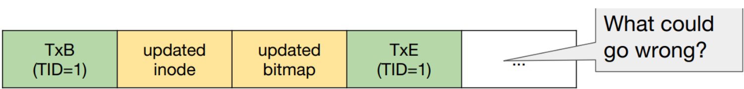
22. Metadata journaling

If we write data after checkpointing metadata, then write data, if crash occurs before all data is written, the inodes will point to garbage data.

How to solve this problem: Write data before writing metadata journal!

write data, wait until it completes

metadata journal write

metadata journal commit

checkpoint metadata

free

If write data fails, then no metadata is written at all, like nothing happened.

If data write succeed, but metadata write fails, still like nothing happened.

If metadata write succeeds, data must be available.

23. Journaling summary

Journaling provides file system consistency

Time complexity of recovery is O(size_of_journal), instead of O(size_of_disk_volume) in fsck.

Widely adopted by most modern file systems, including Linux’s Ext3, Ext4, ReiserFS, IBM’s JFS, SGI’s XFS, and Windows’ NTFS.

Metadata journaling is the most commonly used, since it reduces the amount of traffic to the journal while provide reasonable consistency guarantees.

Key Points

First key point. Brief Answer to questions. (FIXME)

Micro versus monolithnic kernels: Minix and Linux

Overview

Teaching: 0 min
Exercises: 0 min

Questions

The argument of the ages

Objectives

First learning objective. (FIXME)

1. MINIX: what is it?

Developed by Dr. Andrew Tanenbaum in 1984.

UNIX-compatible operating systems for students

Design goals:

Build a UNIX V7 clone that ran on an IBM PC with only a single 360kB floppy disk;

Build and maintain the system using itself, or “self-hosting”;

Make the full source code available to everyone;

Have a clean design students could easily understand;

Make the (micro) kernel as small as possible, since kernel failures are fatal;

Break the rest of the operating system into independent user-mode processes;

Hide interrupts at a very low level;

Communicate only by synchronous message passing with clear protocols; and

Try to make the system port easily to future hardware.

2. MINIX: architecture

Microkernel

Small

Handles interrupts, scheduling, and message passing.

Support API for kernel call.

User programs access kernel calls through system calls.

Device drivers

Runs in user space.

Each controls an I/O device.

Cannot issue I/O instructions directly.

Have to issue instructions via kernel call.

Additional overhead (~500ns)

Enable authorization.

Server processes

Most traditional system calls are located here.

User process send message to servers to request service (i.e., open, read, write, and close files …).

Servers in turn send messages to the corresponding device processes to have these requests performed.

Reincarnation server polls all other server for health report and kill/respawn faulty processes as needed.

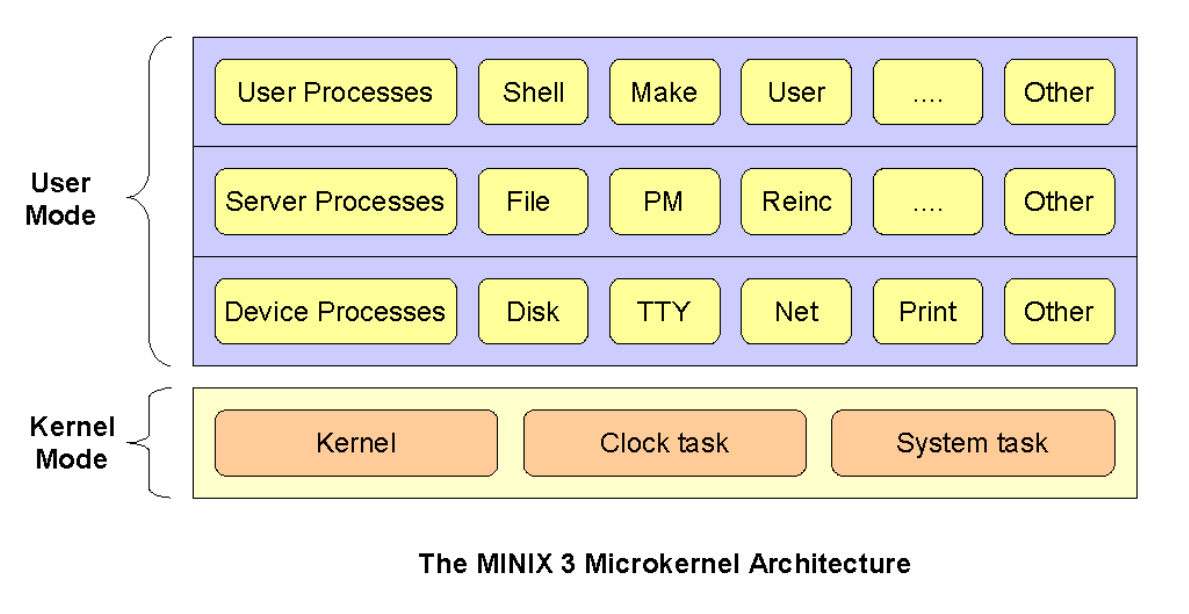
2. MINIX: pros and cons

Advantages

Modularity: the system is well structured and the relationship between the various components is equally well defined.

Security: the combination of the layered system structure and micro-kernel design makes for a architecture that allows for better incorporation of security. Layers 2 – Layer 3 run in User mode while only layer 1, runs in Kernel mode which has all the privileges needed to access any part of the system.

Extensibility: in order to have a functional system, one needs the kernel setup as well as the key services that are needed to start off. All the other functions can be added as and when needed. This makes it simpler to extend and/or specialize the function of the system.

Performance & Stability: most problems that cause instability on a computer system are a result of poor designed and/or poorly compiled drivers and user programs. The microkernel architecture allows these programs to be executed and implemented independent of the core components of the operating system, which means that a failure in any of those programs is not catastrophic to the system. The system is able to maintain uptime, despite errors.

Disadvantages

Complexity: the architecture is complex and hence makes it harder to design in the first place and to evolve as time moves on. The computer industry is probably amongst the fastest moving industry of the global economy and as such there is a real need to adjust to new developments in hardware as well as innovations in software.

Communications and Messaging: the architecture needs fast and efficient communications architecture so as to ensure faster communication between the various processes that are running in their individual address spaces as well as with varied security levels. A poor communications implement would negatively impact on the performance of the system.

3. Linux vs MINIX: the flame war of 1992

Dr. Tanenbaum started it!

Linux is obsolete

It has its own wiki page!.

Dr. Ngo was in 7th grade.

At that time, Linux:

was designed by Linus Torvald, an undergraduate student in Finland.

was inspired by Minix

Linux’s kernel is monolithic

Minux uses microkernel

Andrew Tanenbaum (AT)

Linus Torvald (LT)

AT

Most older operating systems are monolithic, that is, the whole operating system is a single a.out file that runs in ‘kernel mode’ (UNIX, MS-DOS, VMS, MVS, OS/360, MULTICS …).

In a microkernel-based system, in which most of the OS runs as separate processes, mostly outside the kernel. (RC4000, Amoeba, Chorus, Mach, and the not-yet-released Windows/NT).

… among the people who actually design operating systems, the debate is essentially over. Microkernels have won. The only real argument for monolithic systems was performance, and there is now enough evidence showing that microkernel systems can be just as fast as monolithic systems.

MINIX is a microkernel-based system. LINUX is a monolithic style system. This is a giant step back into the 1970s. That is like taking an existing, working C program and rewriting it in BASIC. To me, writing a monolithic system in 1991 is a truly poor idea. MINIX was designed to be reasonably portable, and has been ported from the Intel line to the 680x0 (Atari, Amiga, Macintosh), SPARC, and NS32016. LINUX is tied fairly closely to the 80x86. Not the way to go.

LT

Well, with a subject like this, I’m afraid I’ll have to reply.

True, linux is monolithic, and I agree that microkernels are nicer. From a theoretical (and aesthetical) standpoint Linux looses. What you (AT) don’t mention is that minix doesn’t do the micro-kernel thing very well, and has problems with real multitasking (in the kernel).

The fact is that linux is more portable than minix. It’s true - but not in the sense that ast (AT) means: I made linux as conformant to standards as I knew how (without having any POSIX standard in front of me). Porting things to linux is generally /much/ easier than porting them to minix.

I agree that portability is a good thing: but only where it actually has some meaning. There is no idea in trying to make an operating system overly portable: adhering to a portable API is good enough. The very /idea/ of an operating system is to use the hardware features, and hide them behind a layer of high-level calls. That is exactly what linux does: it just uses a bigger subset of the 386 features than other kernels seem to do. Of course this makes the kernel proper unportable, but it also makes for a /much/ simpler design. An acceptable trade-off, and one that made linux possible in the first place.

AT

A multithreaded file system is only a performance hack. When there is only one job active, the normal case on a small PC, it buys you nothing and adds complexity to the code. On machines fast enough to support multiple users, you probably have enough buffer cache to insure a hit cache hit rate, in which case multithreading also buys you nothing. It is only a win when there are multiple processes actually doing real disk I/O. Whether it is worth making the system more complicated for this case is at least debatable.

MINIX was designed before POSIX, and is now being (slowly) POSIXized as everyone who follows this newsgroup knows. Everyone agrees that user-level standards are a good idea. As an aside, I congratulate you for being able to write a POSIX-conformant system without having the POSIX standard in front of you. I find it difficult enough after studying the standard at great length.

My point is that writing a new operating system that is closely tied to any particular piece of hardware, especially a weird one like the Intel line, is basically wrong. An OS itself should be easily portable to new hardware platforms.
When OS/360 was written in assembler for the IBM 360 25 years ago, they probably could be excused. When MS-DOS was written specifically for the 8088 ten years ago, this was less than brilliant, as IBM and Microsoft now only too painfully realize.

LT

You (AT) admit that some of the errors of minix were that it was too portable: including machines that weren’t really designed to run unix. That assumption lead to the fact that minix now cannot easily be extended to have things like paging, even for machines that would support it. Yes, minix is portable, but you can rewrite that as doesn’t use any features”, and still be right.

A multithreaded file system is only a performance hack. Not true. It’s a performance hack /on a microkernel/, but it’s an automatic feature when you write a monolithic kernel - one area where microkernels don’t work too well. When writing a unix the “obsolete” way, you automatically get a multithreaded kernel: every process does it’s own job, and you don’t have to make ugly things like message queues to make it work efficiently.

The operating system /isn’t/ tied to any processor line: UNIX runs on most real processors in existence. Yes, the /implementation/ is hardware-specific, but there’s a HUGE difference. You mention OS/360 and MS-DOG as examples of bad designs as they were hardware-dependent, and I agree. But there’s a big difference between these and linux: linux API is portable (not due to my clever design, but due to the fact that I decided to go for a fairly-well-thought-out and tested OS: unix.) If you write programs for linux today, you shouldn’t have too many surprises when you just recompile them for Hurd in the 21st century.

The bigger picture

“The way the world was thinking about OS design at the time”.

“UNIX: A history and memoir” by Brian Kernighan.

“It’s important to understand the evolution of the technology that we use and take for granted. The decisions that shaped how that technology developed and thus defined the paths that we took were made by real people, working under the pressures and constraints of the time. The more we know about the history, the the more we can appreciate the inventive genius that led to Unix and perhaps better understand why modern computer systems are as they are. If nothing else, choices that might seem wrong-headed or perverse today can often be seen as natural consequences of what was understood and could be accomplished with the resources available at that time.”

Key Points

First key point. Brief Answer to questions. (FIXME)